ISSN 0101-8205 www.scielo.br/cam
Derivative-free methods for nonlinear programming
with general lower-level constraints*
M.A. DINIZ-EHRHARDT1, J.M. MARTÍNEZ1 and L.G. PEDROSO2 1Department of Applied Mathematics, IMECC-UNICAMP
University of Campinas, 13083-859 Campinas, SP, Brazil 2Department of Mathematics, Federal University of Paraná
81531-980 Curitiba, PR, Brazil
E-mails: {cheti|martinez}@ime.unicamp.br, [email protected]
Abstract. Augmented Lagrangian methods for derivative-free continuous optimization with constraints are introduced in this paper. The algorithms inherit the convergence results obtained by Andreani, Birgin, Martínez and Schuverdt for the case in which analytic derivatives exist and are available. In particular, feasible limit points satisfy KKT conditions under the Constant Posi-tive Linear Dependence (CPLD) constraint qualification. The form of our main algorithm allows us to employ well established derivative-free subalgorithms for solving lower-level constrained subproblems. Numerical experiments are presented.
Mathematical subject classification: 90C30, 90C56.
Key words:nonlinear programming, Augmented Lagrangian, global convergence, optimality conditions, derivative-free optimization, constraint qualifications.
1 Introduction
In many applications one needs to solve finite-dimensional optimization prob-lems in which derivatives of the objective functions or of the constraints are not available. A comprehensive book describing many of these situations has been
#CAM-230/10. Received: 15/VIII/10. Accepted: 05/I/11.
recently published by Conn, Scheinberg and Vicente [9]. In this paper we in-troduce algorithms for solving constrained minimization problems of this class, in which constraints are divided in two levels, as in [1]. The shifted-penalty ap-proach that characterizes Augmented Lagrangian methods is applied only with respect to the upper-level constraints whereas the lower level constraints are explicitly included in all the subproblems solved at the main algorithm. Lower-level constraints are not restricted to the ones that define boxes or polytopes. In general we will assume that derivatives with respect to lower-level constraints are available, but derivatives with respect to upper-level constraints and objective function are not.
The form of the problems addressed in this paper is the following:
Minimize f(x) subject toh(x)=0,g(x)≤0,x ∈. (1)
The setrepresentslower-level constraintsof the form
h(x)=0, g(x)≤0. (2)
In the most simple case,will take the form of ann-dimensional box:
= {x ∈Rn|ℓ≤ x ≤u}. (3)
We will assume that the functions f : Rn → R,h : Rn → Rm,g : Rn →
Rp,h : Rn → Rm,g : Rn → Rp are continuous. First derivatives will be
assumed to exist for some convergence results but they will not be used in the algorithmic calculations at all. It is important to stress that the algorithms pre-sented here do not rely on derivative discretizations, albeit some theoretical convergence results evoke discrete derivative ideas.
We aim to solve (1) using a derivative-free Augmented Lagrangian approach inspired in [1]. Given ρ > 0, λ ∈ Rm, μ ∈ R+p, x ∈ Rn, we define the
Augmented LagrangianLρ(x, λ, μ)by:
Lρ(x, λ, μ)=
f(x)+ρ 2
m X
i=1
hi(x)+
λi
ρ
2 +
p
X
i=1
max
0,gi(x)+
μi
ρ
2
At each (outer) iteration the main algorithm will minimize (approximately) Lρ(x, λ, μ)subject tox ∈ using some derivative-free method and, between outer iterations, the Lagrange multipliers λ, μ and the penalty parameter ρ
will be conveniently updated. The definition (4) corresponds to the well-known PHR (Powell-Hestenes-Rockafellar) [12, 24, 27] classical Augmented Lagran-gian formulation. See, also, [7, 8].
In theglobal optimizationframework one finds an approximate global mini-mizer ofLρ(x, λ, μ)onat each outer iteration. In the limit, it may be proved that a global minimizer of the original problem up to an arbitrary precision is found [5]. Global minimization subalgorithms are usually expensive, but the Augmented Lagrangian approach exhibits a practical property called “preference for global minimizers” [1], thanks to which one usually finds local minimizers with suitable small objective function values if efficient local minimization algo-rithms are used for solving the subproblems. In other words, even if we do not find global minimizers of the subproblems, the global results [5] tend to explain why the algorithms work with the sole assumption of continuity of objective function and constraints.
We conjecture that the effectivity of Augmented Lagrangian tools in deriv-ative-free optimization is associated with the main motivation of the general Augmented Lagrangian approach. Augmented Lagrangian methods are not motivated by Newtonian ideas (which involve iterative resolution of linearized problems associated with derivatives). Instead, these methods are based on the idea of minimizing penalized problems with shifted constraints. The most natural updating rule for the multipliers does not use derivatives at all, as its motivation comes from a modified-displacement strategy [24]. Continuity is the only smoothness property of the involved functions that supports the plausibil-ity of Augmented Lagrangian procedures for constrained optimization.
as-sumption is irrelevant from the theoretical point of view. However it is impor-tant to put in relief that we could use many known derivative-free algorithms to minimize Lρ(x, λ, μ)subject to x ∈ , including directional direct search methods, simplex methods or algorithms based on polynomial interpolation [9]. Sometimes lower-level constraints are easy in the sense that we can deal with them using direct directional search methods. For instance, we can use the MADS algorithm [3, 4], which has been proven to be a very good choice for problems where = I nt(). Although most frequently lower-level
con-straints define boxes or polytopes, more general situations are not excluded at all. Sometimes lower-level constraints cannot be violated, because they involve fundamental definitions or because the objective function may not be defined when they are not fulfilled.
The choice of the algorithm that should be used to solve the subproblems de-pends on the nature of the lower-level constraints. The best known case is when
is ann-dimensional box. We will develop a special algorithm for this case.
The algorithm employs an arbitrary derivative-free box-constraint (or even un-constrained) minimization solver which we complement with a local coordinate search in order to ensure convergence. Whenis defined by linear (equality
or inequality) constraints, the technique of positive generators on cones ([9], Chapter 13) may be employed. See [15, 17, 20].
Assume thatxˉis a feasible point of a smooth nonlinear programming problem whose constraints arehˉi(x) = 0,i ∈ I, gˉj(x),j ∈ J and that the active con-straints atxˉ are (besides the equalities)gˉj(x)≤0, j ∈ J0. LetI1⊆ I,J1⊆ J0.
We say that the gradients∇ ˉhi(xˉ)(i ∈ I1),∇ ˉgj(xˉ)(j∈ J1)arepositively linearly
dependentif
X
i∈I1
λi∇ ˉhi(xˉ)+
X
j∈J1
μj∇ ˉgj(xˉ)=0,
where
λi ∈R∀i∈ I1, μj ≥0∀j∈ J1 and
X
i∈I1 |λi| +
X
j∈J1
μj >0.
is strictly weaker than the Mangasarian-Fromovitz (MFCQ) constraint qualifi-cation [21, 28].
The CPLD condition was introduced in [26] and its status as a constraint qualification was elucidated in [2]. In [1] an Augmented Lagrangian algorithm for minimization with arbitrary lower-level constraints was introduced and it was proved that feasible limit points that satisfy CPLD necessarily fulfill the KKT optimality conditions. The derivative-free algorithms introduced in this paper recover the convergence properties of [1].
In [14], Kolda, Lewis and Torczon proposed a derivative-free Augmented Lagrangian algorithm for nonlinear programming problems with a combina-tion of general and linear constraints. In terms of (1), the set is defined by
a polytope in [14]. The authors use the approach of [7], by means of which inequality constraints are transformed into equality constraints with the addi-tion of slack non-negative variables. Employing smoothness assumpaddi-tions, they reproduce the convergence results of [7]. This means that feasible limit points satisfy KKT conditions, provided that the Linear Independence Constraint Qualification (LICQ) holds. In a more recent technical report [19], Lewis and Torczon used the framework of [1] for dealing with linear constraints in the lower level and employed their derivative-free approach for solving the sub-problems. The proposed algorithm inherits the theoretical properties of [1], which means that the results in [19] are based on the CPLD constraint quali-fication. However, the authors don’t consider nonlinear constraints in the lower level set, which is possible in our approach.
This paper is organized as follows. In Section 2 we recall the method and theoretical results found in [1]. In Section 3 we introduce a derivative-free version of [1] for the case in which the lower-level set is a box. In Section 4 we introduce a derivative-free version of the Augmented Lagrangian method for arbitrary lower-level constraints. Section 5 describes some numerical res-ults. Finally, we make some comments and present our conclusions about this work in Section 6.
Notation
• The canonical basis ofRnwill be denoted{e1, . . . ,en}. • For ally∈Rn,y
+=(max{0,y1}, . . . ,max{0,yn})T.
• N= {0,1, . . .}.
• Ifvis a vector andtis a scalar, the statementv≤tmeans thatvi ≤tfor
all the coordinatesi.
• [a,b]m = [a,b] × [a,b] ×. . .× [a,b]mtimes.
2 Preliminary results
In this section we recall the main algorithm presented in [1] for solving (1) withdefined by (2). We will also mention the convergence theorems that are
relevant for our present research.
Algorithm 1(Derivative-based Augmented Lagrangian)
The parameters that define the algorithm are: τ ∈ [0,1),γ > 1,λmin < λmax,
μmax > 0. At the first outer iteration we use a penalty parameterρ1 > 0 and safeguarded Lagrange multipliers estimatesλˉ1∈Rm andμˉ1∈Rpsuch that
ˉ
λ1i ∈ [λmin, λmax] ∀i =1, . . . ,m and μ1i ∈ [0, μmax] ∀i =1, . . . ,p.
Finally,{εk}is a sequence of positive numbers that satisfies
lim
k→∞εk =0. Step 1. Initialization.
Setk ←1.
Step 2. Solve the subproblem.
Computexk ∈Rnsuch that there existvk ∈Rm, wk ∈Rpsatisfying
k∇Lρk(xk,λˉk,μˉk)+
m
X
i=1
vki∇hi(xk)+
p
X
i=1
wik∇g
i(x k)k ≤ε
k, (5)
wki =0 whenever g
i(x
k) <−ε
k, for alli =1, . . . ,p, (7)
kh(xk)k ≤εk. (8)
Step 3. Estimate multipliers.
For alli =1, . . . ,m, compute
λki+1= ˉλik+ρkhi(xk) (9)
and
ˉ
λki+1∈ [λmin, λmax]. (10)
For alli=1, . . . ,p, compute
μki+1=max{0,μˉki +ρkgi(xk)}, (11)
Vik =max
gi(xk),−
ˉ
μki ρk
,
and
ˉ
μki+1∈ [0, μmax]. (12)
Step 4. Update penalty parameter.
Ifk >1 and
max{kh(xk)k∞,kVkk∞}> τmax{kh(xk−1)k∞,kVk−1k∞},
define
ρk+1=γρk.
Else, define
ρk+1=ρk.
Updatek ←k+1 and go to Step 2.
Lemma 1 below shows that the points xk generated by Algorithm 1 are,
Lemma 1. Assume that{xk}is a sequence generated by Algorithm1. Then, for all k=1,2, . . .we have:
∇f(xk)+ ∇h(xk)λk+1+ ∇g(xk)μk+1+ ∇h(xk)vk+ ∇g(xk)wk≤εk,
where
wk ≥0, wik =0 whenever g
i(x
k) <−ε k,
g
i(x k)≤ε
k ∀i =1, . . . ,p, kh(xk)k ≤εk.
Proof. The proof follows from (5–8) using the definitions (9) and (11).
Lemma 2. Assume that the sequence{xk}is generated by Algorithm1and that K is an infinite sequence of indices such that
lim
k∈Kx k
=x∗.
Suppose that gi(x∗) <0. Then, there exists k0∈ K such that
μki+1=0 for all k ∈K,k ≥k0.
Proof. See the proof of formula (4.10) in Theorem 4.2 of [1].
Theorem 1. Assume that x∗is a limit point of a sequence generated by
Algo-rithm1. Then:
1. If the sequence of penalty parameters{ρk} is bounded, x∗ is a feasible
point of (1). Otherwise, at least one of the following two possibilities holds:
• The point x∗satisfies the KKT conditions of the problem
Minimizekh(x)k22+ kg(x)+k22 subject to h(x)=0, g(x)≤0. • The CPLD constraint qualification corresponding to the lower-level
2. If x∗is a feasible point of(1)then at least one of the following two
possi-bilities holds:
• The KKT conditions of(1)are fulfilled at x∗.
• The CPLD constraint qualification corresponding to all the con-straints of(1)(h(x) = 0,g(x) ≤ 0,h(x) =0,g(x)≤ 0) does not hold at x∗.
Proof. See Theorems 4.1 and 4.2 of [1].
Theorem 1 represents the type of global convergence result that we want to prove for the algorithms presented in this paper. In [1], under additional assumptions, it is proved that the penalty parameters remain bounded when one applies Algorithm 1 to (1). The first part of Theorem 1 says that the algorithm behaves in the best possible way in the process of finding feasible points. This result cannot be improved since the feasible region could be empty and, on the other hand, the algorithm is not equipped for finding global minimizers. It must be observed that, since the lower-level set is generally simple, the CPLD condition related tois usually satisfied at all the lower-level feasible points.
The second part of the theorem (which corresponds to Theorem 4.2 of [1]) says that, under the CPLD constraint qualification, every feasible limit point is KKT. Since CPLD is weaker than popular constraint qualifications like LICQ (regular-ity) or MFCQ (Mangasarian-Fromovitz), this result is stronger than properties that are based on LICQ or MFCQ. The consequence is that, roughly speaking, Algorithm 1 “works” when it generates a bounded sequence (so that limit points necessarily exist). The first requirement for this is, of course, that the conditions (5–8) must be effectively satisfied at every outer iteration, otherwise the algo-rithm would not be well defined. This requirement must be analyzed in every particular case. A sufficient condition for the boundedness of the sequence is the boundedness of the set
{x ∈Rn|g(x)≤ε,kh(x)k ≤ε} for some ε >0.
3 Derivative-free method for box lower-level constraints
In this section we define a derivative-free method that applies to problem (1) whenis a box defined by (3).
Algorithm 2 (Derivative-free Augmented Lagrangian for box constraints in
the lower level)
Letτ ∈ [0,1), γ > 1, λmin < λmax, μmax > 0, ρ1 > 0, λˉ1, μˉ1 and{εk} be
as in Algorithm 1. Steps 1, 3 and 4 of Algorithm 2 are identical to those of Algorithm 1. Step 2 is replaced by the following:
Step 2. Solve the subproblem.
Choose a positive toleranceδk < (ui −ℓi)/2,i =1, . . . ,n,such that
δk ≤min
εk
ρk
, εk
. (13)
Findxk ∈such that, for alli =1, . . . ,n,
xk ±δkei ∈⇒Lρk(x
k±δ
kei,λˉk,μˉk)≥Lρk(x
k,λˉk,μˉk). (14)
Since the algorithm found in [19] handles linear constrained problems, it could also be applied to a box constrained problem. The main difference between this algorithm and Algorithm 2 relies on the choice of the solver for the sub-problem. We encourage the use of any derivative-free technique able to find points satisfying (14), whereas in [19] the authors use Generating Set Search methods for solving the subproblems, taking advantage of the geometry of the linear constraints.
Theorem 2. Assume that∇f,∇h,∇g satisfy Lipschitz conditions on the box
. Then Algorithm2is a particular case of Algorithm1. Moreover:
• The sequence{xk}is well defined for all k and admits limit points.
• If the sequence of penalty parameters {ρk} is bounded, x∗ is feasible.
Otherwise, every limit point x∗ is a stationary point of the box con-strained problem
• If x∗is a feasible limit point, then at least one of the following
possibili-ties holds:
1. The point x∗fulfills the KKT conditions of
Minimize f(x), subject to h(x)=0,g(x)≤0,x ∈.
2. The CPLD constraint qualification is not satisfied at x∗for the
con-straints h(x)=0,g(x)≤0,x ∈.
Proof. By (4), (10), (12) and the Lipschitz assumption, there exists M > 0
such that for allx,y ∈we have:
k∇Lρk(x,λˉk,μˉk)− ∇Lρk(y,λˉk,μˉk)k∞≤ Mρkkx−yk∞. (15)
Assume thatxk is computed at Step 2 of Algorithm 2. Giveni ∈ {1, . . . ,n},
sinceδk < (ui−ℓi)/2, we may consider three possible cases:
• ℓi ≤xik−δk and xik+δk ≤ui;
• ℓi >xik−δk and xik+δk ≤ui;
• ℓi ≤xik−δk and xik+δk >ui.
Consider the first case. By (14) and the Mean Value Theorem, there exists
θik ∈ [−δk, δk]such that
∇Lρk(xk+θike
i,λˉk,μˉk)
i =0.
Then by (15)
[∇Lρk(xk,λˉk,μˉk)]i
≤ Mρkδk. (16) Now consider the second case. By (14) and the Mean Value Theorem, there existsθik ∈ [0, δk]such that
∇Lρk(xk+θike
i,λˉk,μˉk)
i ≥0.
So there existswki ≥0 such that
∇Lρk(x
k
Therefore, by (15),
[∇Lρk(xk,λˉk,μˉk)]i −wik
≤ Mρkδk. (17)
Analogously, in the third case we obtain that there existswik ≥0 such that
[∇Lρk(xk,λˉk,μˉk)]i +wik
≤ Mρkδk. (18)
From (16), (17) and (18), we deduce that there existswk ≥0 such that
∇Lρk(xk,λˉk,μˉk)+
n
X
i=1 ±wkiei
∞
≤ Mρkδk, (19)
where
wik =0 if xik−ℓi ≥δkandxik−ui ≤ −δk.
The sign−takes place in (19) if
xik −ℓi < δk andxik ≤ui−δk,
while the sign+takes place in (19) if
xik−ℓi ≥δk andxik−ui >−δk.
Then, by (13),xksatisfies (5–8) if one redefinesε
k ←max{εk,Mεk}.
To complete the proof of the theorem, observe first that it is always possi-ble to satisfy (14) defining aδk-grid onand takingxk as a global minimizer
ofLρk(x,λˉk,μˉk) on that grid. Sinceis bounded, the sequence is in a com-pact set and limit points exist. Moreover, the box constraints that define
satisfy CPLD, therefore, by Theorem 1, limit points are stationary points of kh(x)k22 + kg(x)+k22. The last part of the thesis is a direct consequence of
Theorem 1.
4 Derivative-free method for arbitrary lower-level constraints
In order to minimize the Augmented Lagrangian subject to the lower-level constraints, we need to use an “admissible” derivative-free algorithm, having appropriate theoretical properties. Roughly speaking, when objective function and constraints are differentiable, an admissible algorithm should compute KKT points of the subproblem up to any required precision.
Let F : Rn → R, h : Rn → Rm, g : Rn → Rp be continuously
differ-entiable. We say that an iterative algorithm is admissible with respect to the problem
MinimizeF(x) subject to h(x)=0,g(x)≤0 (20)
if it does not make use of analytical derivatives of F and, independently ofx0,
it computes a sequence{xν}with the following properties:
• {xν}is bounded;
• Givenε >0 andν1∈N, there existν≥ν1,xν ∈Rn,vν ∈Rm,wν ∈R
p
+,
satisfying:
k∇F(xν)+
m
X
i=1
vνi∇hi(xν)+
p
X
i=1 wiν∇g
i(x
ν
)k ≤ε, (21)
wν ≥0,g(xν)≤ε, (22)
wνi =0 whenever g
i(x
ν
) <−ε, ∀i =1, . . . ,p, (23)
kh(xν)k ≤ε. (24)
In this case, we say thatxν is anε-KKT point of the problem (20).
When we talk about lower-level constraints, we have in mind not only boxes and polytopes, as [14, 15], but also more general constraints that can be handled using, for example, the extreme barrier approach (see [9], Chapter 13). Barrier methods can be useful for solving subproblems when easy inequality constraints define feasible setssuch that
= I nt().
In these cases, incorporating the constraints which definein the upper-level
We will assume that Gρ(x, λ, μ, δ) approximates the gradient of the Aug-mented Lagrangian, in the sense that there existsM>0 such that, for all
x ∈Rn, λ∈ [λmin, λmax]m, μ∈ [0, μmax]p, δ >0,
kGρ(x, λ, μ, δ)− ∇Lρ(x, λ, μ)k ≤δMρ. (25)
Many possible definitions of G can be given satisfying (25) if ∇f,∇h,∇g satisfy Lipschitz conditions. An appealing possibility is to defineGas a simplex gradient [9]. It may not be necessary to use many auxiliary points to compute G because this approximation can be built using previous iterates of the sub-algorithm.
Algorithm 3, defined below, applies to the general problem (1). For this algorithm we will prove that the convergence properties of Algorithm 1 can be recovered under suitable assumptions on the optimization problem. For the ap-plication of Algorithm 3 we will assume that the gradients of the lower-level constraints∇hand∇gare available.
For each outer iterationkwe will denote by{xk,ν}a sequence generated by an admissible algorithm applied to the problem
MinimizeLρk(x,λˉ
k,μˉk) subject to h(x)=0,g(x)≤0. (26)
We assume that the computational form of the admissible algorithm includes some internal stopping criterion that is going to be tested for each ν. When
this stopping criterion is fulfilled we check the approximate fulfillment of (21– 24) without using analytic derivatives of f,h,g. Of course, some admissible
algorithms may ensure that the approximate KKT conditions are satisfied when their convergence criteria are met, in which case it is not necessary to check the approximate KKT conditions.
Algorithm 3(Derivative-free Augmented Lagrangian for general constraints in
the lower level)
Letτ ∈ [0,1), γ > 1, λmin < λmax, μmax > 0, ρ1 > 0, λˉ1, μˉ1 and{εk} be
Step 2. Solve the subproblem.
Choose a toleranceδksuch that
δk ≤
εk
ρk
. (27)
Let{δk,ν}be such thatδk,ν ∈(0, δk]for allνand
lim
ν→∞δk,ν =0.
Step 2.1.Setν←1.
Step 2.2.Computexk,ν.
Step 2.3. Ifxk,ν does not satisfy the intrinsic stopping criterion of the admissi-ble subalgorithm, setν←ν+1 and go to Step 2.2.
Step 2.4. Ifkh(xk,ν)k > εk or there existsi ∈ {1, . . . ,p}such thatgi(xk,ν) >
εk, setν←ν+1 and go to Step 2.2.
Step 2.5.ComputeGρk(xk,ν,λˉk,μˉk, δk,ν),∇h(xk,ν),∇g(xk,ν).
Step 2.6.Define
Iν = {i ∈ {1, . . . ,p} |gi(xk,ν) <−εk}.
Solve, with respect to(v, w), the following problem:
Minimize
Gρk(xk,ν,λˉk,μˉk, δk,ν)+
m
X
i=1
vi∇hi(x k,ν)+
p
X
i=1
wi∇gi(xk,ν)
(28)
subject to w≥0 and wi =0 if i∈ Iν.
Step 2.7.If, at a solution(v, w)of (28) we have that
Gρk(xk,ν,λˉk,μˉk, δk,ν)+
m
X
i=1
vi∇hi(xk,ν)+ p
X
i=1
wi∇g i(x
k,ν )
≤εk, (29)
defineν∗(k) = ν, xk = xk,ν∗(k)
The purpose of Step 2 above is to find a point xk,ν∗(k) and multipliersvk, wk
that verify (5-8), but with the actual gradient of∇Lρk replaced by the simplex gradientGρk. At (28) we compute approximate Lagrange multipliersv, wwith respect to lower-level constraints. In some cases, the basic admissible algorithm may provide these multipliers so that the step (28) may not be necessary. If k ∙ kis the Euclidean norm, (28) involves the minimization of a convex quadratic with non-negative constraints. So, its resolution is affordable in the context of derivative-free optimization, where functions evaluations are generally very expensive, since neither f,gnorhare computed at (28).
In the following theorem we prove that Algorithm 3 is well defined. This amounts to show that the loop defined by Steps 2.1–2.7 necessarily finishes for some finiteν.
Theorem 3. Assume that, for all k = 1,2, . . .an admissible algorithm with respect to (26) is available. Assume, moreover, that the first derivatives of f,h,g, h, g exist and are Lipschitz on a sufficiently large set. Then, Algorithm3 is well defined.
Proof. For fixed k, assume that the admissible algorithm, whose existence
is postulated in the hypothesis, computes a sequence{xk,ν}. Since f,h,ghave Lipschitz gradients, there exists a Lipschitz constant ρkM for the function
∇Lρk(xk,ν,λˉk,μˉk)that is valid for allx in a sufficiently large ball that contains the whole sequence and (25) is satisfied. Letν1be such that
ρkMδk,ν < εk/2 (30)
for allν ≥ ν1 (note that it is not necessary to know the value of M at all). By the definition of admissible algorithm, there exists ν ≥ ν1, vk,ν ∈ Rm,
wk,ν ∈R+p such that:
∇Lρk(xk,ν,λˉk,μˉk)+
m
X
i=1
vik,ν∇hi(xk,ν)+
p
X
i=1
wki,ν∇g
i(x k,ν)
≤εk/2, (31)
g
i(x
k,ν) <−ε
k/2⇒wki,ν =0 for alli =1, . . . ,p, (33)
kh(xk,ν)k ≤εk/2. (34)
Now, by (25) and (30),
kGρk(xk,ν,λˉk,μˉk)− ∇Lρk(xk,ν,λˉk,μˉk, δk,ν)k ≤εk/2.
Thus, by (31),
Gρk(xk,ν,λˉk,μˉk, δk,ν)+
m
X
i=1
vik,ν∇hi(xk)+
p
X
i=1
wki,ν∇g
i(x k)
≤εk,
therefore, by (32–34), the solution of problem (28) necessarily satisfies (29). This means that the loop at Step 2 of Algorithm 3 necessarily finishes in finite
time, so the algorithm is well defined.
Theorem 4. In addition to the hypotheses of Theorem 3, assume that there existsε > 0 such that the set defined by kh(x)k ≤ ε,g(x) ≤ ε is bounded. Then, the sequence{xk} defined by Algorithm3 is well defined and bounded. Moreover, if x∗is a limit point of this sequence, we have:
1. The lower-level constraints are satisfied at x∗(h(x∗)=0,g(x∗)≤0).
2. If the sequence of penalty parameters{ρk} is bounded, x∗ is a feasible
point of (1). Otherwise, at least one of the following two possibilities holds:
• The point x∗satisfies the KKT conditions of the problem
Minimizekh(x)k22+ kg(x)+k22 subject to h(x)=0,g(x)≤0. • The CPLD constraint qualification corresponding to the lower-level
constraints h(x)=0,g(x)≤0does not hold at x∗.
• The KKT conditions of(1)are fulfilled at x∗.
• The CPLD constraint qualification corresponding to all the con-straints of(1)(h(x) =0, g(x) ≤ 0, h(x) =0, g(x) ≤ 0) does not hold at x∗.
Proof. By Theorem 3, the sequence{xk}is well defined. Sinceε
k ≤ εfork
large enough, all the iterates of the method belong to a compact set from some iteration on. This implies that the whole sequence is bounded, so limit points exist.
By (25) we have that:
kGρk(xk,λˉk,μˉk, δk,ν∗(k))− ∇Lρk(xk,λˉk,μˉk)k ≤ Mρkδk,ν∗(k).
Therefore, since, by (27),δk,ν∗(k) ≤δk andρkδk ≤εk,
kGρk(xk,λˉk,μˉk, δk,ν∗(k))− ∇Lρk(xk,λˉk,μˉk)k ≤Mεk.
Then, by (29),
∇Lρk(xk,λˉk,μˉk)+
m
X
i=1
vik∇hi(xk,ν)+
p
X
i=1
wik∇g
i(x k,ν)
≤(1+M)εk.
Moreover, by Step 2 of Algorithm 3,
kh(xk)k ≤εk,g(xk)≤εk
and
wik =0 wheneverg
i(x k
) <−εk.
Therefore, redefiningεk ←(1+M)εk, we have that Algorithm 3 can be seen
as a particular case of Algorithm 1. So the thesis of Theorem 1 holds for
Algo-rithm 3 and the theorem is proved.
may be such admissible algorithm. As we mentioned before, reasonable admis-sible algorithms has been already introduced by several authors for particular classes of lower-level sets. Here we wish to show that, as a last resource, even Algorithm 2 may also be used as admissible algorithm for solving subproblems. The special case of lower-level constraints that we wish to consider is almost as general as it could be. Essentially, we are going to consider arbitrary lower level constraints with bounds on the variables. More precisely, we define:
= {x ∈Rn |h(x)=0,g(x)≤0, ℓ≤x ≤u}, (35)
where h and g are as defined in the Introduction. A very important partic-ular case of (35) is when is described by linear (equality and inequality)
constraints and bounds.
For proving the main admissibility result we will need the following as-sumption.
Assumption A.
If x is a stationary (KKT) point of the problem
Minimizekh(x)k22+ kg(x)+k22 subject to ℓ≤x ≤u then
h(x)=0 and g(x)≤0.
Theorem 5. Assume that F:Rn →Ris continuously differentiable and
sup-pose that h, g,ℓ, u satisfy AssumptionA. Then Algorithm 2is an admissible algorithm for the problem
Minimize F(x)subject to h(x)=0,g(x)≤0, ℓ≤ x ≤u.
Proof. Assume that we apply Algorithm 2 to the problem above. Therefore,
Fplays the role of f,handgstand forhandg, respectively.
Without loss of generality, let us identify {xν}as a convergent subsequence of the sequence generated by Algorithm 2. By Theorem 2, Algorithm 2 is a particular case of Algorithm 1. This implies that, for a givenε >0 andνlarge
enough, condition (21) necessarily holds.
Also by Theorem 2, every limit point is a stationary point of the infeasibility measure subject to the bounds. Therefore, by Assumption A, (22) and (24) also hold forνlarge enough.
Finally, let us prove that (23) also takes place forνlarge enough. Suppose, by
contradiction, that this is not true. Therefore, there existsε >ˉ 0 such that, for allνlarge enough, there exitsi =i(ν)satisfying
g
i(x
ν) <−ˉεandwν
i >0.
Without loss of generality, since the number of different indices ofiis finite, we may assume thati = i(ν)for allν. Hence, in the limit, one has g
i(x
∗) < 0.
Then, by Lemma 2,wiν =0 forνlarge enough. This is a contradiction, which
ends the proof of the theorem.
Theorem 5 shows that Algorithm 2 is an admissible algorithm. Hence, by Theorem 3, it is possible to use Algorithm 2 to generate a sequence{xk,ν}that can be employed in Step 2 of Algorithm 3, when one is attempting to solve (1) withas in (35).
5 Numerical experiments
In this section, we present some computational results obtained with a Fortran 77 implementation of Algorithm 2. Since there is freedom on the choice of the algorithm for the box constrained subproblems, we tested three derivative-free solvers: Coordinate Search [16], the BOBYQA software [25], based on quadratic approximations and trust region techniques, and the well known Nelder-Mead algorithm [22]. In order to satisfy the condition (14), the points returned by BOBYQA or Nelder-Mead are taken as knots of meshes with den-sityδk and, if necessary, other points on these meshes are visited. Eventually,
on the exit of the algorithm. When using the Nelder-Mead algorithm for the subproblems, we force f(x) = ∞ for x 6∈ , to make sure that all
gener-ated points lie within the box. We will call the Augmented Lagrangian with BOBYQA, Nelder-Mead and Coordinate Search as subsolvers, respectively, as AL-BOBYQA, AL-NMead and AL-CSearch.
We say that the Augmented Lagrangian found a solution of a problem if (14) is achieved with tolerance δopt at a point x that is sufficiently feasible,
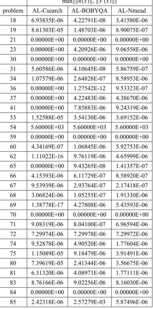
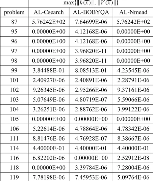
in the sense that, for a tolerance εf eas, max{kh(x)k,kV(x)k} ≤ εf eas. We
consider that the algorithm fails in the attempt of solving the problem in the following cases:
Failure 1: when it cannot find the solution in up to 50 outer iterations,
Failure 2: when it performs 9 outer iterations without improving the feasibility,
Failure 3: when it evaluates the Augmented Lagrangian function more than
106times in a single call of the subsolver.
5.1 Hock-Schittkowski problems
The first set of problems we considered was the Hock-Schittkowski collec-tion [13], which is composed by 119 differentiable problems. We solved only the 47 problems that have general and box constraints simultaneously. The di-mension of the problems varies between 2 and 16, while the number of con-straints are between 1 and 38, exceeding 10 in only 5 cases. We used δopt =
εf eas = 10−5.Table 1 shows the performance of each algorithm for all
prob-lems, with respect to the objective function on the solution, f(x∗),and the
num-ber of function evaluations, f eval, while Table 2 lists the feasibility reached
to 1000 function evaluations and so on. The last three lines show the amount of failures.
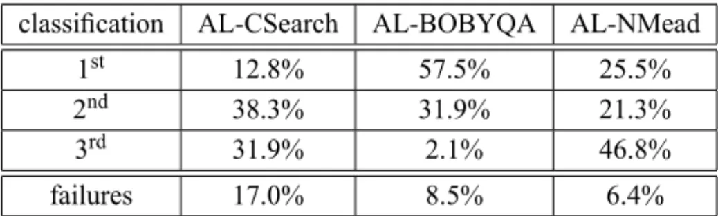
Table 4 shows which method has the best performance for each problem. The first line shows the percentage of problems for which each method evalu-ated less times the Augmented Lagrangian function, the second and third lines consider the occasions where each method was the second best and worst, re-spectively, while the last line informs the total amount of failures.
We can see from the tables that BOBYQA was the most economic subproblem solver. On the other hand, even with the greatest number of function evaluations in many cases, AL-NMead was the most robust. Recall that we do not used the “pure” Nelder-Mead method as a subsolver, but the Nelder-Mead method plus Coordinate Search; the same comment can be made for BOBYQA. AL-CSearch exhibited an intermediate performance when we consider computational effort, but was the least robust among the three algorithms.
5.2 Minimum volume problems
The volume of complex regions defined by inequalities inRd is very hard to
compute. A popular technique, when one needs to compute a volume approx-imation, consists of using a Monte Carlo approach [6, 11]. We will use some small-dimensional examples (d = 2) in order to illustrate the behavior of derivative-free methods in problems in which volumes need to be optimized. In the following examples, one needs to minimize the Monte Carlo approxima-tion of the area of a figure subject to constraints.
Suppose that we want to find the minimal Monte Carlo approximation area of the figure defined by the intersection between two circles that containsnpgiven
points. With this purpose, we draw a tight rectangle containing the intersection of the circles. Then, a large number of points is generated with uniform distribu-tion inside the rectangle. The area of the intersecdistribu-tion is, approximately, the area of the rectangle multiplied by the ratio of random points that dropped inside the intersection of the circles. This is the objective function, the simulated area, that has to be minimized. The constraints arise from the fact that thenppoints have
max{kh(x)k,kV(x)k}
problem AL-Csearch AL-BOBYQA AL-Nmead 18 6.93835E-06 4.22791E-08 3.41580E-06 19 8.61303E-05 1.48703E-06 8.90075E-07 21 0.00000E+00 0.00000E+00 0.00000E+00 23 0.00000E+00 4.20926E-06 9.06558E-06 30 0.00000E+00 0.00000E+00 0.00000E+00 31 5.60586E-06 4.10645E-08 5.86759E-07 34 1.07579E-06 2.64828E-07 8.58953E-06 36 0.00000E+00 1.27542E-12 9.53323E-07 37 0.00000E+00 4.22483E-06 4.38670E-06 41 0.00000E+00 7.85883E-06 9.24319E-06 53 1.52588E-05 3.54130E-06 3.69152E-06 54 5.60000E+03 5.60000E+03 5.60000E+03 59 0.00000E+00 0.00000E+00 0.00000E+00 60 4.34169E-07 1.06845E-06 5.92753E-06 62 1.11022E-16 9.76119E-06 4.65999E-06 65 0.00000E+00 9.43265E-08 1.41357E-07 66 4.15393E-06 6.11729E-07 8.58920E-07 67 9.53939E-06 2.93764E-07 2.17418E-07 68 3.06824E-06 1.05255E-07 1.91330E-06 69 1.38778E-17 4.27808E-06 5.43593E-06 70 0.00000E+00 0.00000E+00 0.00000E+00 71 9.08319E-06 8.04100E-07 6.96594E-06 72 7.29974E-06 7.29978E-06 7.29972E-06 74 9.52878E-06 4.90520E-06 1.77604E-06 75 1.15089E-05 9.18479E-06 3.91491E-06 80 7.39619E-05 2.41344E-06 3.56675E-06 81 6.31320E-06 4.08971E-06 1.77111E-06 83 8.76166E-06 9.02256E-06 8.16030E-06 84 0.00000E+00 0.00000E+00 0.00000E+00 85 2.42318E-06 2.57279E-03 5.87496E-06
max{kh(x)k,kV(x)k}
problem AL-Csearch AL-BOBYQA AL-Nmead 87 5.76242E+02 7.64699E-06 5.76242E+02 95 0.00000E+00 4.12168E-06 0.00000E+00 96 0.00000E+00 4.12168E-06 0.00000E+00 97 0.00000E+00 3.96820E-11 0.00000E+00 98 0.00000E+00 3.96820E-11 0.00000E+00 99 3.84488E-01 8.08513E-01 4.23545E-06 101 2.40927E-06 2.40891E-06 2.28791E-06 102 9.26345E-06 2.95266E-06 9.37161E-06 103 5.07649E-06 4.80719E-07 5.59066E-06 104 3.26251E-06 2.88762E-06 3.99122E-06 105 0.00000E+00 0.00000E+00 0.00000E+00 106 5.22614E-06 4.78864E-06 4.78342E-06 111 8.81476E-06 4.76928E-07 8.38667E-06 114 4.40000E-01 4.40000E-01 4.40000E-01 116 6.82202E-06 0.00000E+00 2.52912E-08 118 0.00000E+00 3.39784E-06 7.28004E-06 119 7.78198E-06 7.45953E-06 5.09764E-06
Table 2 – (continuation).
# of function evaluations AL-CSearch AL-BOBYQA AL-NMead
101to 102 6.4 % 4.3 % 0.0 %
102to 103 17.0 % 34.0 % 21.3 %
103to 104 27.7 % 29.8 % 34.0 %
104to 105 19.1 % 14.9 % 14.9 %
105to 106 12.8 % 8.5 % 10.6 %
106to 107 0.0 % 0.0 % 12.8 %
failure 1 10.6 % 0.0 % 0.0 %
failure 2 0.0 % 2.1 % 0.0 %
failure 3 6.4 % 6.4 % 6.4 %
classification AL-CSearch AL-BOBYQA AL-NMead
1st 12.8% 57.5% 25.5%
2nd 38.3% 31.9% 21.3%
3rd 31.9% 2.1% 46.8%
failures 17.0% 8.5% 6.4%
Table 4 – Comparison of the subsolvers’ performances for 47 problems of Hock-Schittkowski.
a good precision for the simulated area with a small amount of computational effort. We could put the figure of interest inside a very large rectangle, and keep this rectangle fixed within iterations. But, in this case, the computational effort would be possibly bigger.
We considered unions and intersections between three types of figures:
• rectangles, defined by 4 parameters: the coordinates(x,y)of the bottom
left vertex, the height and the width;
• circles, defined by 3 parameters: the coordinates of the center and the radius;
• ellipses, defined by 6 parameters, a,b,c,d,e and f, by the formulae
ax2+2bx y+cy2+d x+ey+ f ≤0.
Suppose that we want the point y to be inside some figure A (or B). This is achieved imposing a constraint of typecA(y) ≤ 0 (orcB(y) ≤ 0). If we want
yto lie inside the intersection between figures A and B, we ask thatcA(y)≤0
andcB(y)≤0,so that each point defines two inequality constraints, 2npat all.
On the other hand, the number of constraints defined by unions arenp, since
each point must be inside figure A or figure B. This is achieved imposing that c(x)=min{cA(x),cB(x)} ≤0.
We firstly considered the problem of minimizing the
1. intersection of two circles,
2. intersection between a rectangle and a ellipse,
3. union of a rectangle and a ellipse and
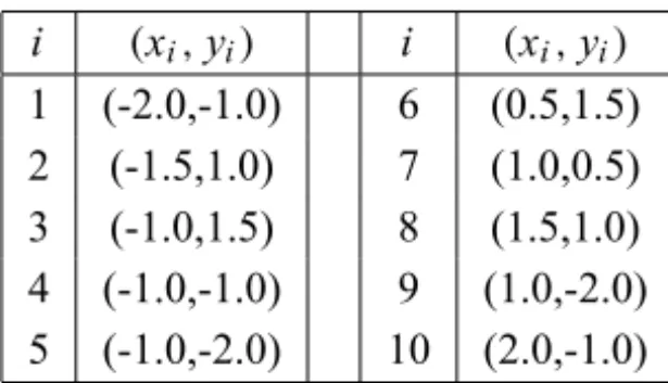
In the four cases the problem consists of finding the smallest intersection (cases 1 and 2) or union (cases 3 and 4) area that contains a given set of points. In all the problems we considered the same set ofnp=10 points given in Table 5.
We adoptedεf eas = δopt = 10−4.The initial guesses for circles and ellipses
were chosen as circles of radius one centered at the origin and for rectangles, squares of side 2 centered at the origin. The value ofnp in our tests is 10, and
the points are
i (xi,yi) i (xi,yi)
1 (-2.0,-1.0) 6 (0.5,1.5) 2 (-1.5,1.0) 7 (1.0,0.5) 3 (-1.0,1.5) 8 (1.5,1.0) 4 (-1.0,-1.0) 9 (1.0,-2.0) 5 (-1.0,-2.0) 10 (2.0,-1.0)
Table 5 – Points that have to be inside the figure whose simulated area is being minimized. The density of points generated in the simulation is 105per unit of area, but the maximum of points allowed is 107. This means that, if the rectangle that contains the desired figure (used in the simulation of the area) has dimensions a×b,then the number of generated points is min{105ab,107}.The initial seeds
used in the random points generator are the same at each call of the simulator, so the simulated area is always the same for the same parameters.
It is simple to find the smallest rectangle that contains a specific rectangle, circle or ellipse. The smallest rectangle that contains a given rectangle is the proper rectangle; for a circle or an ellipse it is the one that is tangent to these figures on four points that can be explicitly found. On the other hand, the area Aof a figure Fcan be simulated generatingngrandom points inside a rectangle
with area AR that contains F and counting the amount of points that lie inside
the figure,ni,so we have that A≈ ARni/ng.We use these two ideas to compute
our objective function according to the following rules:
• In the case of intersection between figures F andG,whereF andGcan be a rectangle, a circle or an ellipse, we compute the smallest rectangles RF andRG that contains each figure, and use the rectangle with smallest
random points inside it and counting the amount of points that lie on F andG. We are using the fact that the intersection of figures F andG is insideRF and is also inside RG.
• In the case of union between two rectangles, a rectangle and a circle or two circles, we add the areas of the figures, since the expression to these areas is well known, and subtract the area of the intersection, which is computed by the method above. We are using the fact that the area of the union is the sum of the area of the figures minus the area of the inter-section.
• In the case of union between a circle and an ellipse, we simulate the area of the figure formed by the ellipse minus the circle, making the simula-tion inside the smallest rectangle that contains the ellipse. We count how many of the random points lie inside the ellipse but outside the circle, so the desired area is approximately the area of the circle plus the simulated area. The same method is used to simulate the area between a rectangle and an ellipse.
• In the case of union between two ellipses, we find the smallest rectangle that contains both ellipses, and simulate the area of the union counting the amount of random points that lie inside the first or the second (or both) ellipse.
Of course, there are many methods to simulate the considered areas, and we are not claiming that the one we chose is the best. More efficient techniques to simulate these areas is a topic under consideration, and can be the scope of future works.
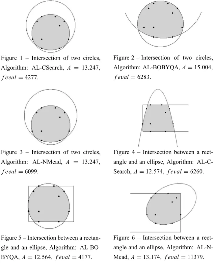
Figures 1–12 show the results obtained in some instances of area problems. The A value is the area of the figure, while f eval is the number of function evaluations performed to find the solution.
rect-Figure 1 – Intersection of two circles, Algorithm: AL-CSearch, A = 13.247,
f eval=4277.
Figure 2 – Intersection of two circles, Algorithm: AL-BOBYQA,A=15.004,
f eval=6283.
Figure 3 – Intersection of two circles, Algorithm: AL-NMead, A = 13.247,
f eval=6099.
Figure 4 – Intersection between a rect-angle and an ellipse, Algorithm: AL-C-Search,A=12.574, f eval=6260.
Figure 5 – Intersection between a rectan-gle and an ellipse, Algorithm: AL-BO-BYQA,A=12.564, f eval=4177.
Figure 6 – Intersection between a rect-angle and an ellipse, Algorithm: AL-N-Mead,A=13.174, f eval =11379.
angle, circle and ellipse, respectively. The last line shows the average area and average number of function calls among all problems.
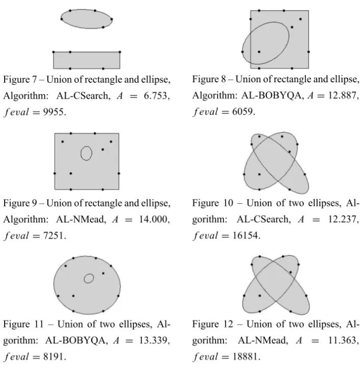
Figure 7 – Union of rectangle and ellipse, Algorithm: AL-CSearch, A = 6.753,
f eval=9955.
Figure 8 – Union of rectangle and ellipse, Algorithm: AL-BOBYQA,A=12.887,
f eval=6059.
Figure 9 – Union of rectangle and ellipse, Algorithm: AL-NMead, A = 14.000,
f eval=7251.
Figure 10 – Union of two ellipses, Al-gorithm: AL-CSearch, A = 12.237,
f eval=16154.
Figure 11 – Union of two ellipses, Al-gorithm: AL-BOBYQA, A = 13.339,
f eval=8191.
Figure 12 – Union of two ellipses, Al-gorithm: AL-NMead, A = 11.363,
f eval=18881.
The impact of the discontinuities decreases with the number of points used in the simulation. (Note that the computer time of function evaluations is propor-tional to that number). Besides, the functionc(x)defined for the union between
area f eval
figure AL-CSearch AL-BOBYQA AL-NMead AL-CSearch AL-BOBYQA AL-NMead
I RR 14.001 13.999 14.003 2709 1535 4959
I RC 12.722 13.467 12.572 6035 3629 7784
I CC 13.247 15.004 13.247 4277 6283 6099
I RE 12.574 12.564 13.174 6260 4177 11379
I CE 13.211 12.973 13.207 5020 7201 11132
I EE 12.058 13.519 13.115 6881 13156 12710
U RR 11.500 12.250 11.499 4312 1745 5717
U RC 13.247 13.894 13.231 2788 874 5466
U CC 13.082 13.890 13.081 2636 4021 4798
U RE 6.723 12.887 14.000 9955 6059 7251
U CE 12.459 13.894 13.333 6715 2042 11688
U EE 12.237 13.399 11.363 16154 8191 18881
average 12.255 13.478 12.985 6145 4909 8989
Table 6 – Results for the minimum area problems.
area were found by the Augmented Lagrangian algorithm with, respectively, Coordinate Search and BOBYQA plus Coordinate Search for the subproblems, and are shown in Figures 7 and 2. In terms of the average area among all fig-ures, shown in the last line of Table 6, AL-CSearch had the best performance, followed by AL-NMead and AL-BOBYQA. On the other hand, AL-BOBYQA required less function evaluations on average, while AL-NMead was the most expensive option.
6 Final remarks
recently introduced methods for constrained optimization when the constraints, generally speaking, admit extreme penalty approaches. Here, we showed that, besides the existing admissible algorithms for solving subproblems, the Aug-mented Lagrangian algorithm with box constraints considered first in this paper (Algorithm 2) may also be considered an admissible algorithm. The practical consequences of this observation remain to be exploited in future research.
From the computational point of view, we introduced a family of Volume Optimization problems, in which we optimize Monte Carlo approximations of volumes subject to constraints. We solved several toy problems of this class, which allowed us to compare different alternatives for solving box-constraint minimization problems in the context of Augmented Lagrangian subproblems without derivatives. We believe that these problems emulate some of the com-mon characteristics of real-life derivative-free optimization problems, especially those originated in simulations.
Acknowledgements. We are indebted to the anonymous referees whose
com-ments helped us to improve the first version of this paper.
REFERENCES
[1] R. Andreani, E.G. Birgin, J. M. Martínez and M. L. Schuverdt,On Augmented Lagrangian Methods with general lower-level constraints.SIAM Journal on Op-timization,18(2007), 1286–1309.
[2] R. Andreani, J.M. Martínez and M.L. Schuverdt, On the relation between the Constant Positive Linear Dependence condition and quasinormality constraint qualification.Journal of Optimization Theory and Applications,125(2005), 473–
485.
[3] C. Audet and J.E. Dennis Jr, Mesh adaptive direct search algorithms for con-strained optimization.SIAM Journal on Optimization,17(2006), 188–217.
[4] C. Audet, J.E. Dennis Jr. and S. Le Digabel, Globalization strategies for Mesh Adaptive Direct Search. Computational Optimization and Applications,46(2010),
193–215.
[6] R.E. Caflisch, Monte Carlo and quasi-Monte Carlo methods, Acta Numerica, Cambridge University Press,7(1998), 1–49.
[7] A.R. Conn, N.I.M. Gould and Ph.L. Toint,A globally convergent Augmented La-grangian algorithm for optimization with general constraints and simple bounds. SIAM Journal on Numerical Analysis,28(1991), 545–572.
[8] A.R. Conn, N.I.M. Gould and Ph.L. Toint.,Trust Region Methods. MPS/ SIAM Series on Optimization, SIAM, Philadelphia (2000).
[9] A.R. Conn, K. Scheinberg and L. N. Vicente, Introduction to Derivative-Free Optimization. MPS-SIAM Series on Optimization, SIAM, Philadelphia (2009). [10] A.L. Custódio and L.N. Vicente,Using sampling and simplex derivatives in pattern
search methods.SIAM Journal on Optimization,18(2007), 537–555.
[11] B.P. Demidovich and I.A. Maron,Computational Mathematics.Mir Publishers, Moscow, (1987).
[12] M.R. Hestenes,Multiplier and gradient methods.Journal of Optimization Theory and Applications,4(1969), 303–320.
[13] W. Hock and K. Schittkowski,Test Examples for Nonlinear Programming Codes. Lecture Notes in Economics and Mathematical Systems, Springer,187(1981).
[14] T.G. Kolda, R.M. Lewis and V. Torczon, A generating set direct search augmented Lagrangian algorithm for optimization with a combination of general and linear constraints. Technical Report, SAND2006–5315, Sandia National Laboratories, (2006).
[15] T.G. Kolda, R.M. Lewis and V. Torczon,Stationarity results for generating set search for linearly constrained optimization. SIAM Journal on Optimization,
17(2006), 943–968.
[16] R.M. Lewis and V. Torczon, Pattern search algorithms for bound constrained minimization.SIAM Journal on Optimization,9(1999), 1082–1099.
[17] R.M. Lewis and V. Torczon,Pattern search algorithms for linearly constrained minimization.SIAM Journal on Optimization,10(2000), 917–941.
[18] R.M. Lewis and V. Torczon,A globally convergent Augmented Lagrangian pattern search algorithm for optimization with general constraints and simple bounds. SIAM Journal on Optimization,12(2002), 1075–1089.
[20] S. Lucidi, M. Sciandrone and P. Tseng, Objective derivative-free methods for constrained optimization. Mathematical Programming,92(2002), 37–59.
[21] O.L. Mangasarian and S. Fromovitz,The Fritz-John necessary optimality condi-tions in presence of equality and inequality constraints.Journal of Mathematical Analysis and Applications,17(1967), 37–47.
[22] J.A. Nelder and R. Mead,A simplex method for function minimization.The Com-puter Journal,7(1965), 308–313.
[23] L.G. Pedroso,Programação não linear sem derivadas.PhD thesis, State Univer-sity of Campinas, Brazil, (2009).
[24] M.J.D. Powell,A method for nonlinear constraints in minimization problems,in Optimization, R. Fletcher (ed.). Academic Press, New York, NY, pp. 283–298, (1969).
[25] M.J.D. Powell,The BOBYQA algorithm for bound constrained optimization
with-out derivatives. Cambridge NA Report NA2009/06, University of Cambridge,
Cambridge, (2009).
[26] L. Qi and Z. Wei,On the constant positive linear dependence condition and its application to SQP methods.SIAM Journal on Optimization,10(2000), 963–981.
[27] R.T. Rockafellar,A dual approach for solving nonlinear programming problems by unconstrained optimization. Mathematical Programming,5(1973), 354–373.
[28] R.T. Rockafellar,Lagrange multipliers and optimality.SIAM Review,35(1993),