ISSN 0101-8205 www.scielo.br/cam
Two derivative-free methods for solving
underdetermined nonlinear systems of equations
N. ECHEBEST1, M.L. SCHUVERDT2∗ and R.P. VIGNAU1 1Department of Mathematics, FCE, University of La Plata
CP 172, 1900 La Plata Bs. As., Argentina
2CONICET, Department of Mathematics, FCE, University of La Plata CP 172, 1900 La Plata Bs. As., Argentina
E-mails: [email protected] / [email protected] / [email protected]
Abstract. In this paper, two different approaches to solve underdetermined nonlinear
sys-tem of equations are proposed. In one of them, the derivative-free method defined by La Cruz, Martínez and Raydan for solving square nonlinear systems is modified and extended to cope with the underdetermined case. The other approach is a Quasi-Newton method that uses the Broyden update formula and the globalized line search that combines the strategy of Grippo, Lampariello and Lucidi with the Li and Fukushima one. Global convergence results for both methods are proved and numerical experiments are presented.
Mathematical subject classification: Primary: 65H10; Secondary: 90C57.
Key words: underdetermined nonlinear systems, Quasi-Newton method, derivative-free line
search, spectral step length, global convergence.
1 Introduction
We consider the problem of determining a solution x∗ ∈ Rn that verifies the
nonlinear system of equations
F(x)=0 (1)
where F : Rn → Rm is a continuously differentiable function and m ≤ n,
the Jacobian matrix of F, denoted by J(x), is not available or requires a pro-hibitive amount of storage. This situation is common when functional values come from experimental measures, for example: from physics, chemistry or economics.
Such kind of problems also appears as the feasible set of general nonlinear programming problems. Our main motivation is the application of the pro-posed methods as subalgorithms for finding feasible points in derivative-free nonlinear programming algorithms such as, for example two-phases algorithms [3, 8, 16, 26], feasible methods [1, 12, 18, 19, 20, 22, 23, 24, 25] and inexact restoration methods [15, 17].
The resolution of square nonlinear systems without using derivatives has been addressed using the spectral residual approach in [11] and the Broyden Quasi Newton approach in [13]. Some ideas of those papers are incorporated in the present work. In [11], the authors defined the derivative-free spectral algorithm for nonlinear equations called DF-SANE. Furthermore, global convergence was proved by using a derivative-free line search that combines the nonmonotone strategy of Grippo, Lampariello and Lucidi [9] with the Li and Fukushima scheme [13].
In [13], a Quasi Newton method based on the Broyden update formula and on a nonmonotone derivative-free line search was defined for the square case. Also in [4] an inexact Quasi-Newton method was introduced with a similar line search technique to the one introduced in [13] and using Bk = J(xk)
periodi-cally. Under appropriate hypotheses, global and superlinear convergence were proved in both papers.
In the present paper we define two approaches for the nonsquare system of equations based on the ideas appearing in [11] and [13]. The proposed algo-rithms use a generalization of the derivative-free nonmonotone line search defined in [11]. The search direction in [11] is computed using the residual vectorF(xk)and the spectral coefficient [2]. For the underdetermined system, the current point is computed by considering a fixed number of Lm directions
Broyden update formula for matrices. It is well established in the literature that, for the square case, this is the most used secant approximation to the Jaco-bian and it works very well locally [6]. As we mentioned before, the Broyden update formula has been previously used by Li and Fukushima and combined with a derivative-free line search for the square case. In [13] the current direc-tion is the soludirec-tion to the linear system
Bkd+F(xk)=0 (2)
and the update matrixBk+1is defined as
Bk+1= Bk+βk
(yk−Bksk)skT kskk2
(3)
whereyk = F(xk)−F(xk−1),sk = xk −xk−1and the parameter βk is chosen such that |βk −1| ≤ ˉβ < 1 for which Bk+1 is nonsingular. In this paper, when there is a solution of the linear system (2) we use such solution as a search direction and, when there is none, we solve the linear system approxi-mately as proposed in [14]. Consequently, we avoid the necessity of choosing the parameterβk.
Under appropriate hypotheses, global convergence of the sequence gener-ated by both methods will be proved. The global convergence result obtained for the algorithm based on the spectral ideas extends the convergence result in [11]. For the Quasi Newton method that uses the Broyden update formula, we obtain convergence using a Dennis-Moré type condition. We show that this condition can be dropped out for a particular derivative-free line search. Thus, both algorithms can be viewed as extensions of the well known methods de-fined in [11] and [13] for square nonlinear systems.
We consider the usual continuously differentiable merit function f:Rn →R,
which consists in a measure of the residualF(x)atx, f(x)= 12kF(x)k2. The iterative algorithms generate a sequence {xk}, for k = 1,2, . . ., start-ing from a given initial point x0. A subsequence of {xk} will be indicated by
{xk}k∈K whereK is some infinite index set.
DF-SANE Algorithm of [11] for handling efficiently problem (1) and we prove the global convergence results. In Section 4 we define the Quasi Newton method using the Broyden update formula and the derivative-free line search introduced in Section 2. We analyze the conditions under which it is possible to obtain global convergence. Both algorithms are tested and the numerical results are presented in Section 5. Finally, some conclusions are drawn in Section 6.
Notation.
• k.kdenotes the Euclidean norm.
• Given a matrixB ∈Rm×n,N(B)denotes the null space of the matrixB.
• Fori =1, . . . ,n; ei is the canonical vector inRn.
• Indenotes the identity matrix inRn×n.
• g(x)=J(x)TF(x)= ∇(1
2kF(x)k 2).
2 The nonmonotone line search without derivatives
In this section we shall be concerned with the nonmonotone derivative-free line search that will be used in the methods defined in the following sections. As we mentioned before, the strategy is based on the line search proposed in [11]. Given the current iteratexk and a search directiondk, the algorithm looks for a
steplengthαk such that
f(xk+αkdk)≤ max
0≤j≤M−1 f(xk−j)+ηk−γ α 2
k f(xk) (4)
whereMis a nonnegative integer, 0< γ <1 and
∞
X
k=0
ηk =η <∞.
This procedure combines the well known nonmonotone line search strat-egy for unconstrained optimization introduced by Grippo, Lampariello and Lucidi [9]:
f(xk+αkdk)≤ max
0≤j≤M−1 f(xk−j)+γ αk∇f(xk)
Td
k, (5)
with the Li-Fukushima derivative-free line search scheme [13]:
kF(xk+αkdk)k ≤(1+ηk)kF(xk)k −γ αk2kdkk
2
The combined strategy (4) produces a robust nonmonotone derivative-free line search that takes into account the advantages of both schemes. The line search (4) is strongly based on the fact that the search direction comes from the residual vector. For details we refer to [11]. In such paper this strategy was implemented and tested using an extensive set of numerical experiments which showed its competitiveness for square systems of nonlinear equations.
In this paper, given a general search direction dk, based on (5) and (6), we
consider the following line search condition:
f(xk+αkdk)≤ max
0≤j≤M−1 f(xk−j)+ηk−γ α 2
kkdkk
2
, (7)
wherekdkk2takes the place of f(x
k)in (4), obtaining a more general strategy.
For completeness, we establish here the implemented process.
Algorithm 1. Nonmonotone line search
Given d ∈ Rn, 0 < τ
min < τmax < 1, 0 < γ < 1, M ∈ N, {ηk} such that
ηk >0and P∞
k=0ηk =η <∞
Step 1: Compute fk =max{f(xk), . . . , f(xmax{0,k−M+1})}
α+=α−=1
Step 2: If f(xk +α+d)≤ fk+ηk−γ α+2kdk
2,
define dk =d,αk =α+, xk+1=xk+αkdk else if f(xk−α−d)≤ fk+ηk−γ α2−kdk
2,
define dk = −d,αk =α−, xk+1=xk+αkdk else
chooseα+new ∈ [τminα+, τmaxα+],α−new ∈ [τminα−, τmaxα−]
α+=α+new,α−=α−new and go to step 2
Proposition 2.1. Algorithm1is well defined.
Proof. See Proposition 1 of [11].
Algorithm 2. General Algorithm
Given x0, F(x0), M ∈ N,0 < τmin < τmax <1,0 ≤ ǫ < 1,0 < γ <1,{ηk}
such thatηk >0and ∞
X
k=0
ηk =η <∞.
Set k ←0.
Step 1: IfkF(xk)k ≤ ǫmax{1,kF(x0)k}stop. Step 2: Compute a search direction dk.
Step 3: Findαk and xk+1=xk+αkdk using Algorithm 1. Update k←k+1and go to Step 1.
By considering the procedure above it is possible to obtain results (see be-low) that will be used in the next sections for obtaining the convergence results. The proofs of Propositions 2.2 and 2.3 below follow from Propositions 2 and 3 in [11] updated for the line search condition (7). We establish them here for completeness.
Proposition 2.2. For all k∈Nconsider
Uk =max{f(x(k−1)M+1), . . . , f(xk M)}
and defineν(k)∈ {(k−1)M+1, . . . ,k M}the index for which f(xν(k))=Uk. Then for all k=1,2, . . .
f(xν(k+1))≤ f(xν(k))+η
whereη= ∞
X
i=0
ηi.
Proof. We have that
f(xk M+1) ≤ max{f(x(k−1)M+1), . . . , f(xk M)} +ηk M−γ α2k Mkdk Mk
2
= Uk+ηk M−γ α2k Mkdk Mk
2≤
Uk+ηk M
then
f(xk M+2) ≤ max{f(x(k−1)M+2), . . . , f(xk M+1)} +ηk M+1−γ α2k M+1kdk M+1k2
Thus, by an induction argument we obtain:
f(xk M+l)≤Uk+ l−1 X
j=0
ηk M+j −γ α2k M+l−1kdk M+l−1k2,
forl =1,2, . . ..
Sinceν(k+1)∈ {k M+1, . . . ,k M+M}
Uk+1= f(xν(k+1))≤Uk+ M−1 X
j=0
ηk M+j−γ αν(2k+1)−1kdν(k+1)−1k2.
Thus, for allk=1,2, . . .we have that
f(xν(k+1))≤ f(xν(k))+
M−1 X
j=0
ηk M+j −γ α2ν(k+1)−1kdν(k+1)−1k2≤ f(xν(k))+η
as we wanted to prove.
Proposition 2.3.
lim
k→∞α
2
ν(k)−1kdν(k)−1k2=0. Proof. For allk=1,2, . . . we have
f(xν(k+1))≤ f(xν(k))+
M−1 X
j=0
ηk M+j −γ αν(2k+1)−1kdν(k+1)−1k2.
Writing the last inequality fork = 1,2, . . . ,L and adding theseL inequali-ties we obtain
f(xν(L+1))≤ f(xν(1))+
(L+1)M−1 X
j=M
ηj−γ L
X
j=1
α2ν(j+1)−1kdν(j+1)−1k2.
Therefore
γ L
X
j=1
αν(2j+1)−1kdν(j+1)−1k2≤ f(xν(1))+
(L+1)M−1 X
j=M
ηj − f(xν(L+1))
Thus, the series
∞
X
j=1
α2ν(j+1)−1kdν(j+1)−1k2is convergent and
lim
k→∞α
2
ν(k)−1kdν(k)−1k2=0
as claimed.
Proposition 2.4. The sequence {xk} generated by the General Algorithm is contained in
= {x ∈Rn: f(x)≤ f(xν(1))+η}.
Proof. From Proposition 2.2 we have that, for allk ≥1,
f(xν(k+1))≤ f(xν(1))+η.
Therefore, f(xk+1)≤ f(xν(k+1))≤ f(xν(1))+ηas we wanted to prove. The results obtained up to here depend strongly on the line search technique without taking into account the way in which the directiondkin the step 2 of the
Algorithm 2 was computed.
From now on we will consider the set
K = {ν(1)−1, ν(2)−1, ν(3)−1, . . .} (8)
and from Proposition 2.3 we have that
lim
k∈Kα
2
kkdkk2=0. (9)
Observe that from the proof of Propositions 2.3 and 2.4 we obtain the following result:
Proposition 2.5. If we take M =1in Algorithm1then
• the sequence {xk} generated by the General Algorithm is contained in = {x ∈Rn: f(x)≤ f(x
0)+η}.
• the series ∞
X
k=1
αk2kdkk
3 Derivative-Free Spectral Algorithm for solving Underdetermined Non-linear Equations (DF-SAUNE)
In this section, we develop a derivative-free method based on the algorithm DF-SANE [11] updated for the underdetermined case. DF-DF-SANE is a derivative-free method for solving square nonlinear systems that uses then−dimensional residual vector as a search direction together with a spectral step length and a globalization strategy that produces a nonmonotone process. The spectral coefficient is the inverse of an approximation of the Rayleigh quotient with respect to a secant approximation of the Jacobian:
σk = hsk,ski hyk,ski
, (10)
whereyk =F(xk)−F(xk−1),sk =xk−xk−1, see [2, 11].
The iterative process in DF-SANE can be viewed as a Quasi Newton method considering the matrix Bk = σ1
kIn together with the iteration xk+1 = xk −
αkBk−1F(xk)=xk−αkσkF(xk)whereαk is computed using the derivative-free
nonmonotone strategy (4).
In order to solve the underdetermined case we propose to combine the idea of the augmented Jacobian algorithm, see for example [29], with the spectral residual vector explained above. In order to do that we consider Lm as the ceil
number ofmn, that is,
Lm =
n
m if
n m ∈N hn
m i
+1 if not.
For each j = 0, . . . ,Lm −1 we define the matrices Ej ∈ Rm×n as
fol-lows. IfLm = mn thenEj is the matrix whose rows are themcanonical vectors ej m+1,ej m+2, . . .,ej m+m inRn. If Lm = [mn] +1 then for j =0, . . . ,Lm−2, Ej is the same matrix defined above and ELm−1 is the matrix whose rows are
themcanonical vectorse(Lm−1)m+1, . . . ,en,e1, . . .,eLmm−ninR
n.
Givenxk, for j =0, . . . ,Lm −1 we consider the directiondk+j ∈Rnas the
solution to the square linear system 1
σk+j
Ej Vj
dk+j =
−F(xk+j)
0
where Ej was defined above,Vj ∈ R(n−m)×n is the matrix whose rows are the
canonical vectors in Rn that span N(Ej) and σk+j is a spectral coefficient.
Thus we can observe thatdk+j = −σk+j ETj F(xk+j)and
kdk+jk2=|σk+j |2kF(xk+j)k2. (12)
Once the directiondk+j is obtained, the line search is performed using
Algo-rithm 1.
Observe that the system (11) is a square system that resembles the one used in DF-SANE for obtaining its current direction.
Given an arbitrary initial pointx0∈Rn, the algorithm that allows us to obtain the next iterate is given below:
Algorithm 3. DF-SAUNE
Given x0, F(x0),0< γ <1,0< τmin< τmax<1,σ0=1, 0< σmin< σmax<∞,0≤ǫ <1.
Set k ←0.
Main Step: Given xk, F(xk),σk.
(1) IfkF(xk)k ≤ ǫmax{1,kF(x0)k}, stop. (2) For j =0:Lm −1
• Compute dk+j = −σk+j ETj F(xk+j)
• Findαj and xk+j+1=xk+j +αjdk+j using the Algorithm 1. • IfkF(xk+j+1)k ≤ ǫmax{1,kF(x0)k}, stop.
• Compute s =xk+j+1−xk+j, y =F(xk+j+1)−F(xk+j)andσ =
hEjs,Ejsi
hy,Ejsi .
• If|σ| ∈ [σmin, σmax]defineσk+j+1 =σ. If not, chooseσk+j+1
such that|σk+j+1| ∈ [σmin, σmax]
End
(3) Update k←k+Lmand repeat the main step.
By (9) we have that
lim
k∈Kα
2
kkdkk2=0.
Thus, using (12) and considering that each|σk| ∈ [σmin, σmax]we obtain that lim
k∈Kα
2
k f(xk)=0. (13)
In the following Theorem we prove the main convergence result associated to DF-SAUNE Algorithm. The proof follows the idea of the Theorem 1 in [11] updated for the Algorithm 3.
Theorem 3.1. Assume that {xk}k∈Nis the sequence generated by Algorithm3.
Then, for every limit point x∗of{x
k}k∈Kthere exists an index j0∈ {0, . . . ,Lm−1} such that
hJ(x∗)TF(x∗),ETj 0F(x
∗)i =0 (14)
Proof. Letx∗ be a limit point of{xk}k∈K. Thus, there is an infinite index set
K1⊂ K such that
lim
k∈K1
xk =x∗.
Then, by (13),
lim
k∈K1
αk2f(xk)=0. (15)
We have two possibilities:
(1) The sequence{αk}k∈K1 does not tend to zero;
(2) The sequence{αk}k∈K1 tends to zero.
In the first case there exists an infinite sequence of indicesK2⊂ K1such that
αk ≥c>0 for allk ∈ K2. Then, by (15), lim
k∈K2
f(xk)=0.
Since f is continuous this implies that f(x∗)=0.
Suppose that case 2 happens. Once the directiondkwas computed, in the step
2 of the Algorithm 1, one tests the inequality
f(xk+α+dk)≤ ˉfk+ηk−2γ α+2σ
2
If this inequality does not hold, one tests the inequality
f(xk−α−dk)≤ ˉfk+ηk−2γ α−2σ
2
k f(xk). (17)
The first trial points at (16)–(17) are α+ = α− = 1. Since lim
k∈K1
αk = 0,
there existsk0 ∈ K1such thatαk < 1 for allk ∈ K1,k ≥ k0. Therefore, for those iterationsk, there are stepsαk+ andαk− that do not satisfy (16) and (17) respectively for which
lim
k∈K1
α+k = lim
k∈K1
α−k =0.
So, for allk ∈K1,k ≥k0, we have that
f(xk+αk+dk) > fˉk+ηk−2γ (α+k)2σk2f(xk), (18) f(xk−αk−dk) > fˉk+ηk−2γ (αk−)
2σ2
k f(xk). (19)
Since|σk| ∈ [σmin, σmax], we have that (18) implies
f(xk+α+kdk) > fˉk+ηk−γ (αk+)
2f(xk) (20)
and (19) implies
f(xk−α−kdk) > fˉk+ηk−γ (αk−)
2f(xk) (21)
whereγ =2γ σ2 max.
The inequality (20) implies that
f(xk+αk+dk) > f(xk)−γ (α + k)
2
f(xk).
So,
f(xk+α+kdk)− f(xk) >−γ (αk+)
2f
(xk).
By Proposition 2.4,{f(xk)}is a sequence bounded above by a constantC >0.
Thus,
f(xk +αk+dk)− f(xk)≥ −γC(α+k)
2 (22)
which implies that
kF(xk+αk+dk)k
2− kF(x
k)k2≥ −γC(αk+)
So,
kF(xk+α+kdk)k2− kF(xk)k2
αk+ ≥ −γCα
+ k.
By the Mean Value Theorem, there existsξk ∈ [0,1]such that
hg(xk +ξkα+kdk),dki ≥ −γCαk+.
SinceLmis finite there exists j0∈ {0, . . . ,Lm−1},K2⊂ K1such that, for all
k∈ K2
dk = −σk
ETj
0 V T j0
F(xk) 0
!
.
Thus, we have that
−σk
g(xk+ξkα+kdk),
ETj0 VjT0
F(xk) 0
!
≥ −γCαk+.
Now, ifσk >0 for infinitely many indicesk ∈ K2the last inequality implies that, fork∈ K2,k≥k0
g(xk +ξkα+kdk),
ET
j0 V T j0
F(xk) 0
!
≤ γCα + k
σk ≤
γCαk+ σmin
. (23)
Using (21) and proceeding in the same way, we obtain that, for k ∈ K2,
k≥k0,
g(xk−ξ ′ kα
− kdk),
ETj0 VjT0
F(xk) 0
!
≥ −Cγ α − k
σk ≥ −
Cγ αk− σmin
. (24)
for someξk′ ∈ [0,1].
Since{σk}and{f(xk)}are bounded we have that{kdkk}is bounded.
Then, using thatα+k → 0, αk− → 0, and taking limits in (23) and (24), we obtain that
g(x∗),
ETj
0 V T j0
F(x∗) 0
!
=0.
Remark 3.2. We have proved that there exists an index j0 ∈ {0, . . . ,Lm−1}
such that the gradient ofkF(x)k2atx∗is orthogonal to the residual ET j0F(x
∗).
Note that whenm = n, the result of Theorem 3.1 coincides with the conver-gence result obtained in [11]. Thus, we can say that DF-SAUNE Algorithm is an extension of DF-SANE.
Corollary 3.3. Assume that x∗is a limit point of the sequence{xk}k∈K gener-ated by Algorithm3and suppose that for all j ∈ {0, . . . ,Lm−1}we have that hJ(x∗)ETjv, vi 6=0for allv∈Rn, v6=0. Then F(x∗)=0.
4 Derivative-Free Quasi Newton method using the Broyden update for-mula (DF-QNB)
In this section we will define a Quasi Newton method based on the Broyden update formula for the matrices with the derivative-free line search defined in Algorithm 1 and we will establish the convergence results.
We will define the search direction as an approximate solution to the linear system Bkd = F(xk)and we will use the nonsquare rank one Broyden update
formula:
Bk+1= Bk+
(yk−Bksk)skT sT
k sk
(25)
wheresk =xk+1−xk and yk = F(xk+1)−F(xk).
As previously stated, the aim is to solve the linear system accurately when it is possible and in an approximate way in any other case, as considered in [14].
Algorithm 4. DF-QNB
Given x0, B0 ∈ Rm×n, F(x0),0 < γ < 1, 0 ≤ θ0 < 1, 1 > 0, 0 < τmin <
τmax<1,0≤ǫ <1.
Set k ←0.
Step 2.1: Find d such that
Bkd+F(xk)=0 and kdk ≤1. (26)
If such direction d is found, define dk = d, θk+1 = θk and go to
Step 3.
Step 2.2: Find a solution d ofmin
d∈RnkBkd+F(xk)k.
If d satisfies
kBkd+F(xk)k ≤θkkF(xk)k and kdk ≤1 (27)
define dk =d,θk+1=θk and go to Step 3.
Else, set dk =0, xk+1=xk,θk+1= θk2+1and go to Step 5. Step 3: Findαk and xk+1=xk+αkdk using Algorithm 1.
Step 4: Update Bk+1using(25).
Step 5: Update k ←k+1and go to Step 1.
In [14], the subproblems in Step 2 were defined using two different matrices.
Remark 4.1. Whenm =nthe Algorithm 4 is similar to the Algorithm defined in [13], in the sense that both of them use the Broyden update formula. In [13] the authors solve the linear system (2) by using the update (3). We acknowledge that, in large scale problems, it is difficult to solve linear systems, even when they do have a solution. Having that in mind we have tried to find an approximate solution in the sense of (27) for those cases.
The following theorems establish the necessary hypotheses for obtaining the convergence results.
Theorem 4.2. Assume that Algorithm 4 generates an infinite sequence {xk}. Suppose that
lim
k→∞h(Bk−J(xk))dk,F(xk)i =0 (28) and there exists k0∈Nsuch that, for all k ≥k0, θk =θ <1. Then, every limit
Proof. Letx∗be a limit point of{xk}k∈K, then there existsK1 ⊂ K such that lim
k∈K1
xk =x∗.
We know that lim
k∈Kα
2
kkdkk2=0, so lim k∈K1
α2kkdkk2=0.
We will consider two cases: a) lim
k∈K1
αk 6=0 andb) lim
k∈K1
αk =0. Let suppose the first case. Then, we have that
lim
k∈K1
kdkk =0. (29)
(1) First we assume that in the process of the Algorithm 4, the direction dk
was calculated finitely times solving the linear systemBkd+F(xk)=0.
Then, there exists k1 ∈ K1 such that ∀k ≥ k1,k ∈ K1, dk verifies
the formula kBkd + F(xk)k ≤ θkkF(xk)k. Thus, for all k ∈ K1, k≥max{k0,k1}we have that
hBkdk,F(xk)i ≤ θ2−1
2 kF(xk)k 2. This implies that
h(Bk−J(xk))dk,F(xk)i + hJ(xk)dk,F(xk)i ≤ θ2−1
2 kF(xk)k 2
.
Taking limits fork ∈K1,k ≥max{k0,k1}in the last expression, and using the continuity ofF andJ and (28)–(29), we obtain that
0≤ θ
2
−1 2 kF(x
∗)k2.
Sinceθ <1, we have thatkF(x∗)k =0 as we wanted to prove.
(2) Let assume now that the direction dk was obtained infinitely many times
solving the linear systemBkd+F(xk)=0.
Then, there existsK2⊂ K1such that for allk ∈ K2we have that Bkdk + F(xk)=0.
Thus, for allk ∈ K2,
Taking limits fork ∈ K2,k ≥k0and using the continuity ofFand J and (28)–(29), we obtain that
kF(x∗)k =0.
Let suppose the caseb). Since the sequence{dk}k∈Nis bounded (and then it
is bounded inK1), there exists K2⊂K1anddˉ ∈Rnsuch that lim
k∈K2
dk =d.
In the line search, to choose the step αk the algorithm DF-QNB tests the following inequalities
f(xk+α+dk)≤ fk+ηk−γ α+2kdkk
2 (30)
f(xk−α−dk)≤ fk+ηk−γ α2−kdkk
2. (31)
The initial values ofα+andα−are 1. Since lim
k∈K2
αk =0, there existsk ∈ K2 such thatαk <1 for allk ∈ K2,k ≥ k. Thus, for those iterations kthere exist stepsαk+ andαk−that do not satisfy (30) and (31) and lim
k∈K2
αk+ = lim
k∈K2
α−k =0. So we have that
f(xk+α+kdk) > fk+ηk−γ (α + k)
2kd
kk2 (32)
f(xk−αk−dk) > fk+ηk−γ (α − k)
2kdkk2
. (33)
Considering (32), the following inequality holds
f(xk+αk+dk) > fk+ηk−γ (α + k)
2k
dkk2> f(xk)−γ (αk+)2kdkk2.
Sincekdkk ≤1we obtain that
f(xk+α+kdk)− f(xk)
αk+ >−γ α
+ k1
2.
By the Mean Value Theorem there exists ξk+∈ [0,1]such that
hg(xk+ξk+α +
k dk),dki>−γ α + k1
2. (34)
Considering (33), we have that
f(xk−αk−dk) > fk+ηk−γ (α − k)
2kd
kk2> f(xk)−γ (αk−)
2kd
Sincekdkk ≤1we obtain that
f(xk−α−kdk)− f(xk)
αk− >−γ α
− k1
2.
By the Mean Value Theorem there existsξk−∈ [0,1]such that
hg(xk−ξk−α −
kdk),dki< γ α−k1
2
. (35)
Taking limits in (34) and (35) whenk → ∞,k∈ K2, we obtain that
hg(x∗),di = hJ(x∗)TF(x∗),di =0.
Thus,
hJ(x∗)d,F(x∗)i =0. (36)
Now, as we did before, we have to consider two cases: (i) the direction dk
was calculated finitely many times solving the linear system Bkd +F(xk) =
0; and (ii) dk was obtained infinitely many times solving the linear system Bkd+F(xk)=0.
Proceeding in analogous way as we did when lim
k∈K1
αk 6= 0 and using (28) and (36) we obtain that
kF(x∗)k =0
as we wanted to prove.
Observe that, according to Proposition 2.4, we have thatkF(xk)kis bounded.
Thus, if
lim
k→∞
k(Bk −J(xk))dkk kdkk
=0
we obtain the hypothesis (28). The last condition is known as a necessary and sufficient condition for obtainingq-superlinear convergence of classical Quasi Newton methods [6].
If we can not guarantee thatθk = ˉθ < 1 for k ≥ k0 then we can prove the following result which is similar to one obtained in [14].
Theorem 4.3. Suppose that, in Algorithm 4, θk is increased infinitely many times and define
Assume that
lim
k∈K∗
kBk−J(xk)k =0. (37)
Then, every limit point x∗of the sequence{x
k}k∈K∗ is a solution of(1)or it is a global minimizer ofkF(x∗)+J(x∗)(x −x∗)k.
Proof. IfF(x∗)=0 we are done. Let us assume thatkF(x∗)k>0. Suppose
thatx∗is not a global minimizer ofkF(x∗)+ J(x∗)(x −x∗)k, therefore, there existsdsuch thatkdk ≤ 12 and
kF(x∗)+J(x∗)dk<kF(x∗)k
thus
kF(x∗)+J(x∗)dk
kF(x∗)k ≤r <1.
By (37) and the continuity ofF andJ, we have that
kF(xk)+Bk(x∗−xk+d)k
kF(xk)k ≤
r +1
2 (38)
for allk large enoughk ∈ K∗. But, sincekdk ≤ 12 and lim
k∈K∗xk = x
∗we have
that, for all large enoughk ∈ K∗,kx∗−xk+dk ≤1. So, (38) contradicts the
fact that: θk →1 and a direction verifying (27) can be obtained. A pointx∗that is a global minimizer of the functionkF(x∗)+J(x∗)(x−x∗)k
can be viewed as the solution of the linear least squares problem
min
x∈RnkA(x−x
∗
)−bk (39)
where A = J(x∗) andb = −F(x∗). The linear function is the affine model of the function F around x∗. We can not expect, in general, to find x∗ such that F(x∗) = 0 since the problem could not have a solution. Likewise, we
can not expect to find x∗ such that F(x∗)+ J(x∗)(x −x∗) = 0 since this is an underdetermined linear system of equations and J(x∗) could not have full
4.1 Analysis of the case M =1
In this subsection we analyze the case in which the derivative-free line search used in Algorithm DF-QNB considers M = 1. By the presence ofηk the line search is still nonmonotone but it imposes an almost monotone behavior of the merit function when xk is close to a solution. Thus, M = 1 is plausible
considering we are working with a Quasi Newton method. M =1, as pointed out in [11], could be inconvenient for the spectral residual method because it performs highly nonmonotone even in a neighborhood of an isolated solution.
Next, we will demonstrate that, in this case, our algorithm verifies the assump-tion (28).
Firstly, under this case, using Proposition 2.5 it can be observed that
∞
X
k=1
kskk2= ∞
X
k=1
αk2kdkk2<∞. (40)
Secondly, it will be convenient to define the matrix
Ak+1= Z 1
0
J(xk+tsk)dt.
Thus,Ak+1sk =yk and
Bk+1=Bk+
(Ak+1−Bk)skskT kskk2
.
Finally, we can use the result that appears in Lemma 2.6 of [13] and that we present here for completeness.
Lemma 4.4 (Lemma 2.6, [13]). Let us suppose that the set = {x ∈ Rn : f(x) ≤ f(x0)+η} is bounded and that J(x) is Lipschitz continuous in .
If(40)is verified then
lim
k→∞
1
k k−1 X
i=0
ρi2=0 where
ρk = k(Ak+1−Bk)dkk kdkk
.
Thus, we can prove the following convergence result.
Theorem 4.5. Assume that Algorithm4generates an infinite sequence{xk}, that M = 1in the line search and that the hypotheses of Lemma4.4hold. Then, if there exists k0such thatθk = ˉθ < 1for all k ≥ k0, there is a limit point x∗ of
{xk}k∈Nthat is a solution of(1).
Proof. By Proposition 2.5 we have that (40) holds. Thus, by Lemma 4.4, there is a subsetK˜ ⊂Nsuch that
lim
k∈ ˜K
k(Ak+1−Bk)dkk
kdkk
=0. (41)
Letx∗be a limit point of the subsequence{xk}k∈ ˜K. Note that
| h(Bk−J(xk))dk,F(xk)i |≤ k(Bk−J(xk))dkk kF(xk)k
≤(k(Ak+1−Bk)dkk + k(J(xk)−Ak+1)dkk)kF(xk)k.
By Proposition 2.5 we have that kF(xk)k is bounded. Thus, taking limit
whenk ∈ ˜K,k → ∞and using that {dk}is bounded and (41), we obtain that
k(Ak+1−Bk)dkk → 0. Also, by definition of Ak+1we obtain that k(J(xk)−
Ak+1)dkk → 0. Thus, we prove that (28) happens for k ∈ ˜K and the proof
follows from Theorem 4.2.
Observe that this particular line search improves the results of Theorem 4.2.
5 Numerical experiments
In this section we present some computational results obtained with a Fortran 77 implementation of DF-SAUNE and DF-QNB algorithms. All experiments were run on a personal computer with INTEL(R) Core (TM) 2 Duo CPU E8400 at 3.00 GHz and 3.23 GB of RAM.
5.1 Test problems
The problems used for these numerical experiments, of the form F(x) = 0,
F :Rn → Rm,m ≤n, were a set of problems defined by feasible sets of
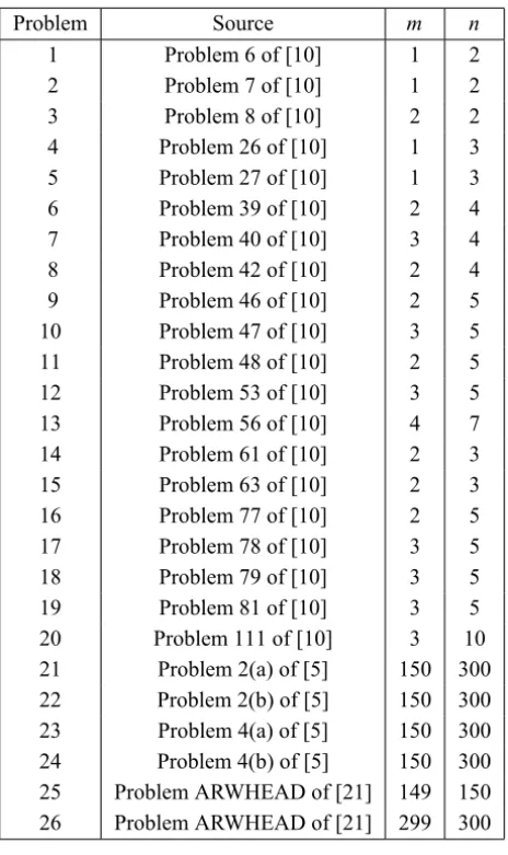
non-linear programming problems in Hock and Schittkowski [10], where the number of variables ranges from 2 to 10, and the number of equations from 1 to 4. Also, conceiving tests for larger dimension problems, we tested some problems described in [5]. Some of the test problems analyzed here have been previously examined in [7] for problems with bound constraints and using derivatives in order to achieve similar results to those pursued here; that is, to solve under-determined nonlinear systems.
In Table 1 we show the data of the problems. In column 1 we show the number of the problem, in column 2 the source of the problem and in the last columns the number of equations (m) and variables (n).
Initial points were the same as in the cited references.
Remark 5.1. The case (a) in Problems 2 and 4 of [5] corresponds to the use of the initial point x0(1 : n) = 2. The case (b) in Problem 2 and 4 of [5] corresponds to the use ofx0(1:n)=150 as initial point.
5.2 Implementation
In the implementations of DF-SAUNE and DF-QNB algorithms:
1. The parameters for Algorithm 1 were:
M=2,τmin=0.1,τmax=0.5,γ =10−4,η0=1, • ∀k ∈N,k ≥1 ηk = kF(x0)k
2k for small size problems.
• ∀k ∈N,k ≥1, ηk = kF(x0)k
(1+k)2 for medium size problems. 2. The parameters for DF-SAUNE Algorithm were:
ǫ=10−6,σ0=1,σmin=10−10,σmax=1010. 3. The parameters for DF-QNB Algorithm were:
ǫ=10−6,θ
Problem Source m n
1 Problem 6 of [10] 1 2
2 Problem 7 of [10] 1 2
3 Problem 8 of [10] 2 2
4 Problem 26 of [10] 1 3
5 Problem 27 of [10] 1 3
6 Problem 39 of [10] 2 4
7 Problem 40 of [10] 3 4
8 Problem 42 of [10] 2 4
9 Problem 46 of [10] 2 5
10 Problem 47 of [10] 3 5
11 Problem 48 of [10] 2 5
12 Problem 53 of [10] 3 5
13 Problem 56 of [10] 4 7
14 Problem 61 of [10] 2 3
15 Problem 63 of [10] 2 3
16 Problem 77 of [10] 2 5
17 Problem 78 of [10] 3 5
18 Problem 79 of [10] 3 5
19 Problem 81 of [10] 3 5
20 Problem 111 of [10] 3 10
21 Problem 2(a) of [5] 150 300 22 Problem 2(b) of [5] 150 300 23 Problem 4(a) of [5] 150 300 24 Problem 4(b) of [5] 150 300 25 Problem ARWHEAD of [21] 149 150 26 Problem ARWHEAD of [21] 299 300
Table 1 – Data of the problems.
4. In DF-QNB, the first B0matrix was computed by finite differences as an aproximation to the Jacobian matrix inx0.
5. In DF-QNB, we have used ACCIM algorithm described in [27] to find a solution to Bkd = −F(xk). For solving the least squares problem
min
kdk≤1kBkd+F(xk)k
2we have used BVLS algorithm described in [28]. 6. The stopping condition for the two new algorithms was:
7. The maximum number of function evaluations allowed was: • M A XF E =5000, for small size problems,
• M A XF E =15000, whenn=150,
• M A XF E =30000, whenn=300.
For DF-QNB method we have also added the required evaluations to cal-culate the initial matrixB0.
The implementation of NEWUOA is the original version of M.J.D. Powell [21] with its stopping criterion, that is, the algorithm stops when the trust-region radius is lower than a toleranceρend =10−6. As previously mentioned, NEWUOA algorithm solved the least squares problem minkF(x)k2in our trials.
5.3 Numerical results
In Table 2 we show the results obtained by DF-SAUNE (DF-S) and DF-QNB (DF-B) algorithms taking into account the final valuekF(xend)kand the number function evaluations. The results correspond to the stopping criterion satisfac-tion or to internal condisatisfac-tions that do not allow further improvement.
Table 2 also shows the number of problems (column 1), the number of itera-tions (Iter, column 2), the number of function evaluaitera-tions (Feval, column 3), and the final functional values obtained for both codes (kF(xend)k, column 4).
These results illustrate DF-QNB effectiveness, although DF-SAUNE has also a satisfactory behavior. We can see in 15 out of the 20 test problems DF-QNB used less function evaluations than DF-SAUNE. It is also worth mentioning that when DF-QNB requires more function evaluations than DF-SAUNE such difference becomes particulary significant. These problems are too small to consider useful showing CPU time readings.
In problem 5, we have seen that, in many interations the norm of the solution
dk of the linear system Bkd +F(xk) = 0 is bigger than 1and, in those
iter-ations, DF-QNB has to solve subproblem (27). Because of that, the decrease of the merit function kF(x)k is very slow and the algorithm requires many functional evaluations.
Iter Feval kF(xend)k
Problem
DF-S DF-B DF-S DF-B DF-S DF-B
1 83 4 85 7 2.555333D-08 1.460382D-08
2 44 62 70 844 5.616128D-08 8.074138D-06
3 52 10 54 19 1.852329D-07 1.029118D-06
4 49 61 85 929 1.487057D-07 1.188074D-07
5 1 251 2 4815 0.0D+00 1.341756D-06
6 57 30 105 76 5.707520D-08 3.311382D-08
7 122 5 327 10 8.140108D-09 7.144642D-09
8 56 15 137 20 9.481413D-09 8.774760D-07
9 143 19 448 25 9.368079D-08 8.287063D-06
10 80 8 133 14 1.483448D-08 6.553991D-07
11 1 1 4 7 0.0D+00 5.264796D-06
12 1 1 3 7 0.0D+00 1.026234D-09
13 92 5 163 13 5.098483D-08 3.366883D-07
14 101 10 206 22 3.382254D-08 1.863196D-09
15 67 7 134 16 7.382254D-08 2.947364D-07
16 54 10 125 16 3.911728D-07 2.765711D-07 17 318 6 1176 12 2.243582D-06 1.839195D-07
18 68 7 169 13 6.362777D-08 1.753428D-06
19 696 8 5000 14 1.137512D-01 1.641720D-08 20 132 12 461 29 1.200486D-08 4.219128D-09
Table 2 – Small size problems.
allowed. We believe that the bad perfomance of DF-SAUNE it is related to the strategy used to define the matrices Ej when mn ∈/ N. We think that it is an
interesting future work to study a better strategy to complete the last matrix Ej
in that specific case.
In Table 3 we show the number of iterations, number of function evaluations and the CPU time in seconds required by DF-SAUNE, DF-QNB and NEWUOA algorithms running the medium size problems 21, 22, 23, 24, 25 and 26. In that table we indicate the number of equations (m) and variables (n) of the problems. Firstly, an overall review of the numerical results shows that final residual values are similar for all tested methods.
Problem Method Iter Feval kF(xend)k CPU
DF-SAUNE 105 123 1.096064D-06 0.01
21 DF-QNB 2 303 4.544647D-11 0.05
NEWUOA 3768 5765 4.681655D-10 245.12 DF-SAUNE 440 566 1.656464D-08 0.04
22 DF-QNB 1 302 2.002649D-05 0.05
NEWUOA 4010 6043 4.284213D-10 270.10 DF-SAUNE 147 185 5.481636D-06 0.01
23 DF-QNB 128 649 4.283559D-06 2.43
NEWUOA 15472 30000 8.203095D-07 1286.79 DF-SAUNE 94 122 9.933035D-07 0.01
24 DF-QNB 394 731 7.489404D-05 9.67
NEWUOA 18874 29205 1.334399D-07 1248.00 DF-SAUNE 3476 9848 2.696620D-07 0.34
25 DF-QNB 13 164 3.628420D-05 4.23
NEWUOA 7533 15000 1.092628D-09 124.15 DF-SAUNE 3001 8664 1.393098D-06 0.33
26 DF-QNB 13 314 5.139963D-05 52.20
NEWUOA 15072 30000 1.453638D-08 1237.54 Table 3 – Medium size problems.
time for DF-SAUNE was always substantially shorter than the one for DF-QNB. The reason is that DF-QNB algorithm has to solve a linear system of equations or a least squares problem in every iteration.
Finally we ran the well known NEWUOA solver in order to measure the number of function evaluations of our algorithms. Although NEWUOA was designed to solve unconstrained optimization problems, we can conclude that our methods performs satisfactorily.
6 Conclusions
on the Broyden Quasi Newton method. The algorithms can be viewed as gen-eralizations of the algorithms defined in [11] and [13], the last one combined with [14].
From a theoretical point of view we were able to obtain some convergence results. Under usual assumptions on the Jacobian matrix we establish global convergence of the scheme that uses the spectral residual idea. This convergence result can be seen as the underdetermined counterpart of the result presented in [11] for the square case.
For the Broyden Quasi Newton method we obtain global convergence under a Dennis Moré type condition. We have shown that this condition can be dropped out for a particular line search. It remains a challenge to reduce the restrictive hypotheses required in Theorem 4.3 of Section 4.
Numerical experiments suggest that the algorithms behave as expected. We consider both approaches are promising even though we also believe that it is necessary to test a more challenging set of problems in order to decide which is more suitable. Furthermore, such decision could depend on the requirements of each user.
Since many nonlinear programming problems have also box constraints, future research will consider the extension of this type of algorithms to solve under-determined nonlinear systems with bound constraints.
Acknowledgements. The authors are indebted to two anonymous referees and to the Guest Editor for their careful reading of this paper.
REFERENCES
[1] J. Abadie, J. Carpentier, Generalization of the Wolfe Reduced-Gradient Method
to the Case of Nonlinear Constraints. Optimization, Edited by R. Fletcher,
Academic Press, New York (1968), 37–47.
[2] J. Barzilai and J.M. Borwein, Two-point stepsize gradient methods. IMA J. of Numerical Analysis,8(1988), 141–148.
[3] R.H. Bielschowsky and F.A.M. Gomes,Dynamic control of infeasibility in
[4] E.G. Birgin, N. Kreji´c and J.M. Martínez, Globally convergent inexact
quasi-Newton methods for solving nonlinear systems. Numerical Algorithms,32(2003),
249–260.
[5] N. Dan, N. Yamashita and M. Fukushima, Convergence properties of inexact
Levenberg-Marquardt method under local error bound conditions. Opt. Methods
and Software,17(2002), 605–626.
[6] J.E. Dennis and R.B. Schnabel,Numerical Methods for Unconstrained
Optimiza-tion and Nonlinear EquaOptimiza-tions. Prentice-Hall, Englewood Cliffs, 1983.
[7] J.B. Francisco, N. Kreji´c and J.M. Martínez, An interior point method for solving
box-constrained underdetermined nonlinear systems. J. of Comp. and Applied
Math.,177(2005), 67–88.
[8] N.I.M. Gould and Ph. L. Toint, Nonlinear programming without a penalty func-tion or a filter. Math. Prog.,122(2010), 155–196.
[9] L. Grippo, F. Lampariello and S. Lucidi, A nonmonotone line search technique
for Newton’s method. SIAM J. on Numerical Analysis,23(1986), 707–716.
[10] W. Hock and K. Schittkowski,Test Examples for Nonlinear Programming Codes. Springer Series Lectures Notes in Economics Mathematical Systems, (1981). [11] W. La Cruz, J.M. Martínez and M. Raydan, Spectral residual method
with-out gradient information for solving large-scale nonlinear systems of equations.
Mathematics of Computation,75(2006), 1429–1448.
[12] L.S. Lasdon, Reduced Gradient Methods. Nonlinear Optimization 1981, edited by M.J.D. Powell, Academic Press, New York (1982), 235–242.
[13] D.H. Li and M. Fukushima, A derivative-free line search and global
conver-gence of Broyden-like method for nonlinear equations. Opt. Meth. and Software,
13(2000), 181–201.
[14] J.M. Martínez,Quasi-Inexact Newton methods with global convergence for
solv-ing constrained nonlinear systems. Nonlinear Analysis,30(1997), 1–7.
[15] J.M. Martínez, Inexact Restoration method with Lagrangian tangent decrease
and new merit function for nonlinear programming. J. of Opt. Theory and
Appli-cations,111(2001), 39–58.
[16] J.M. Martínez, Two-Phase Model Algorithm with Global Convergence for
Non-linear Programming. J. of Opt. Theory and Applications,96(1998), 397–436.
[17] J.M. Martínez and E.A. Pilotta, Inexact Restoration algorithms for constrained
[18] A. Miele, H.Y. Huang and J.C. Heideman,Sequential Gradient-Restoration Algo-rithm for the Minimization of Constrained Functions, Ordinary and Conjugate
Gradient Version. J. of Opt. Theory and Applications,4(1969), 213–246.
[19] A. Miele, A.V. Levy and E.E. Cragg, Modifications and Extensions of the
Con-jugate-Gradient Restoration Algorithm for Mathematical Programming Problems.
J. of Opt. Theory and Applications,7(1971), 450–472.
[20] A. Miele, E.M. Sims and V.K. Basapur, Sequential Gradient-Restoration Algo-rithm for Mathematical Programming Problems with Inequality Constraints, Part
1, Theory. Rice University, Aero-Astronautics Report No. 168 (1983).
[21] M.J.D. Powell, The NEWUOA software for unconstrained optimization without
derivatives. Nonconvex Opt. and its Applications,83(2006), 255–297.
[22] M. Rom and M. Avriel,Properties of the Sequential Gradient-Restoration
Algo-rithm (SGRA), Part 1: Introduction and Comparison with Related Methods. J. of
Opt. Theory and Applications,62(1989), 77–98.
[23] M. Rom and M. Avriel Properties of the Sequential Gradient-Restoration
Algo-rithm (SGRA), Part 2: Convergence Analysis. J. of Opt. Theory and Applications,
62(1989), 99–126.
[24] J.B. Rosen, The Gradient Projection Method for Nonlinear Programming, Part
1, Linear Constraints. SIAM J. on Applied Math.,8(1960), 181–217.
[25] J.B. Rosen, The Gradient Projection Method for Nonlinear Programming, Part
2, Nonlinear Constraints. SIAM J. on Applied Math.,9(1961), 514–532.
[26] J.B. Rosen,Two-Phase Algorithm for Nonlinear Constraint Problems. Nonlinear Prog. 3, Edited by O.L. Mangasarian, R.R. Meyer and S.M. Robinson, Academic Press, London and New York (1978), 97–124.
[27] H.D. Scolnik, N. Echebest, M.T. Guardarucci and M.C. Vacchino, Incomplete
Oblique Projections for Solving Large Inconsistent Linear Systems. Math. Prog.
B,111(2008), 273–300.
[28] P.B. Stark and R.L. Parker, Bounded Variable Least Squares: An Algorithm and
Applications. J. Computational Statistics,10(1995), 129–141.
[29] H.F. Walker and L.T. Watson, Least-Change secant update methods for