ISSN 0101-8205 www.scielo.br/cam
Duality results for stationary problems of open pit mine
planning in a continuous function framework
A. GRIEWANK and N. STROGIES
Institute of Mathematics of the Humboldt-Universität zu Berlin, DFG Research Center Matheon Mathematics for Key Technologies E-mails: [email protected] / [email protected]
Abstract. Open Pit Mine Planning problems are usually considered in a Mixed Integer Pro-gramming context. Characterizing each attainable profile by a continuous function yields a con-tinuous framework. It allows for a more detailed modeling of slope constraints and other material properties of slanted layers. Although the resulting nonlinear programming problems are in general non-convex and non-differentiable, they provide certain advantages as one can directly compute sensitivities of optimal solutions w.r.t. small data perturbations. In this work duality results are derived for the stationary problems of the continuous framework employing an addi-tional condition called convex-likeness.
Mathematical subject classification: 49N15, 26B25, 90C26, 90C31.
Key words: Duality, convex-likeness, continuous optimization, Mine planning, calculus of variations.
1 Introduction
In the continuous framework for Open Pit Mine planning any profile is described by a continuous function. A profilepis called feasible if it satisfies the Dirichlet boundary condition p(x)− p0(x)=0 forx ∈∂, the nonnegativity condition
p(x)− p0(x)≥0 for allx ∈and the so called slope constraint 3p(x)=lim sup
ˆ x→x← ˜x
|p(xˆ)−p(x˜)|
k ˆx − ˜xk ≤ω(x,p(x)) (1)
with an upper semi continuous parameterω. By construction,3p(∙)is an upper
semi continuous functional ([11, Theorem 9.2]). The feasible set P ⊂ C()
contains all those profiles. The stationary Capacitated Final Open Pit Problem (CFOP) for a given effort constraintE ∈R+reads
min −G(p) s.t. p ∈P
ˆ
E(p) ≤0
(CFOP)
withEˆ(p)=E(p)−Eand
G(p) ≡
Z
p(x)
Z
p0(x)
g(x, τ )dτd x
E(p) ≡
Z
p(x)
Z
p0(x)
e(x, τ )dτd x
representing the gain generated by a certain profile p and the effort which is necessary to create it. Here, the densities g,e ∈ L∞( × Z) are only as-sumed to be essentially bounded and the effort density has to be strictly pos-itive, i.e. e(x,z) ≥ e0 > 0 which is a natural assumption. For the analy-sis of general optimization problems in Banach spaces one normally needs at least continuous Fréchet differentiability or convexity of the objective func-tional and the constraint mapping [8]. Problem (CFOP) usually exhibits nei-ther continuous Fréchet differentiability (consequence of [2, Proposition 5(ii)] as Gateaux differentiability is necessary for Fréchet differentiability) nor con-vexity (consequence of [2, Lemma 1] as this property is obtained only for rather artificial choices ofω).
Although certain additional assumptions on the parameters of the model ensure these properties, they are not taken into account in this work.
as the parameterω can only be derived by geostatistic tools and hence carry uncertainties about the exact value. Because the mapping representing the slope condition is expected to be neither differentiable nor convex an alternative to the concepts named above needs to be applied. As it is not even expected to be Lipschitz continuous the direct application of subdifferential calculus will not yield satisfactory results either.
The article reviews duality results for so called convex-like optimization prob-lems [8, 9] as these cover a slightly wider class of probprob-lems than the properly convex ones. It is organized as follows.
Section 2 recalls the basic definitions needed for the analysis of convex-like optimization problems. Moreover basic duality theorems for this class will be given. It closes with the presentation of a characterization of solutions as saddle points of the Lagrange functional.
Section 3 applies the duality theory for convex-like optimization problems to the problem formulation of (CFOP) presented above with p ∈ P being
con-sidered as an implicit hard constraint, i.e. the optimization is done by only considering feasible profiles. This formulation is a continuous analog to the well known discrete ones as the values for ω are prescribed and hence equal some kind of pointwise predecessor relation. Moreover an example shows that the characteristic convex-likeness is not generally given. The section closes with a more general theorem which covers at least some instances of the type given in the example.
In Section 4 the stability constraint is included as a non-implicit constraint in the optimization process. After the definition of the corresponding range space of the constraint and the appropriate dual space we may apply again duality results for convex-like optimization problems.
2 Preliminaries
In general an optimization problem defined on a Banach space Xis given by
min F(x) s.t. g(x)∈ −CY
x ∈ ˆS
where F : X → R is the objective functional, g : X → Y a vector space valued constraint mapping withY being partially ordered by some coneCY and
ˆ
Sis a nonempty subset of X. To justify the investigation of (P) the feasible set S= {x ∈ ˆS|g(x)∈ −CY}is assumed to be nonempty as well. Problem (P) will
be referred to asprimal problemthroughout.
A more intuitive access for this problem is obtained when (P) is reformulated as a penalized optimization problem given in terms of
min
x∈ ˆS sup
y∈CY∗
F(x)+ hy,g(x)i. (P′)
HereCY∗ ≡ {y ∈ Y∗|hy,xi ≥ 0 for allx ∈ CY}represents the so calleddual
conew.r.t. the duality pairingh∙,∙iY∗,Y. Throughout the indices Y∗,Y will be
left out as it will be clear from the context for which spaces the pairings are considered.
While if (P) and (P′) are not equivalent in general, it is well known that this is guaranteed if the ordering coneCY is closed (e.g., see [8, Lemma 6.5]). Now
one introduces thedual problemof (P′) as
max
y∈CY∗infx∈ ˆS
F(x)+ hy,g(x)i. (D)
For any feasible elementx˜ ∈ Sof the primal problem and any feasible element of the dual problemyˆ ∈C∗one obtains the weak duality relation
inf
x∈ ˆS
F(x)+ h ˆy,g(x)i ≤ F(x˜).
Definition 2.1 (convex-like). LetSbe a nonempty subset of a vector space X.
Moreover letY be a partially ordered vector space with ordering coneCY.
A mapping gˆ : S → Y is calledconvex-likeif the set Mg = ˆg(S)+CY is
convex inY.
The concept of convex-likeness indeed covers slightly more functions than the ones just being convex. For example consider the functiong:R→R2,g(x)= (si n(x),x) which is convex-like w.r.t. the positive orthant but obviously not convex. The next step for the introduction of duality results is to ensure of a constraint qualification. As it is well known, the Slater condition was originally defined for convex problems but can be generalized to convex-like problems as well.
Definition 2.2 (generalized Slater condition). Problem (P) satisfies the gener-alized Slater condition(GSC) if there existsx ∈ ˆSsuch thatg(x)∈ −i nt(CY).
The following duality result applies the definitions introduced above and can be found in [8, Theorem 6.7].
Theorem 2.1 (Duality Theorem applying convex-likeness). Consider an op-timization problem of form(P). Moreover, let the ordering cone CY be closed
and contain interior points, i.e. i nt(CY) 6= ∅. Furthermore, let the mapping
(F,g) : ˆS → R×Y be convex-like w.r.t. the ordering cone R+×CY in the
product spaceR×Y .
If (P) is solvable and the generalized Slater condition holds, there exist a solution of the dual problem(D)as well and the extremal values of both prob-lems coincide.
Essentially, the proof uses the convexity of the set
M =(F,g)(Sˆ)+R+×CY
and the fact, that due to the generalized Slater condition this set contains in-terior points. We may thus apply the classical Eidelheit separation theorem ([7, Theorem 1.3]) on i nt(M) and (F(x∗),0Y) with x∗ being the optimal
One speaks of strong duality when (P) and (D) have solutions whose optimal values coincide. For optimal solutions of (P) the following characterization can be given where the proof is adapted from [6, Corollary 5.3].
Theorem 2.2 (characterization of solutions).Consider a problem of form(P). Moreover let the composite mapping(F,g): ˆS→R×Y be convex-like w.r.t.
the product coneR+ ×CY, CY be closed with i nt(CY) 6= ∅ and (GSC) be
satisfied.
Then the following assertions are equivalent
(i) x is an optimal solution ofˉ (P)
(ii) ∃ ˉy ∈CY∗ s.t. (xˉ,yˉ)is a saddle point of the Lagrange functional L(x,y)= F(x)+ hy,g(x)i
in the sense of L(xˉ,y)≤ L(xˉ,yˉ)≤ L(x,yˉ)for all x,y∈S×C∗
Y.
Proof. (i)⇒(ii)
By Theorem 2.1 the dual problem is solvable and the extremal values coincide. Hence one has
min
x∈ ˆS sup
y∈CY∗
F(x)+ hy,g(x)i ≤ F(xˉ)+ h ˉy,g(xˉ)i ≤ max
y∈CY∗infx∈ ˆS
F(x)+ hy,g(x)i
Bygˆ(xˉ)∈ −CY and the definition of the infimum it follows
L(xˉ,y)≤ L(xˉ,yˉ)≤L(x,yˉ) i.e. the Lagrange functional admits a saddle point.
(ii)⇒(i)
AsL admits an saddle point in(xˉ,yˉ)it follows hy,gˆ(xˉ)i ≤ h ˉy,gˆ(xˉ)i∀y∈CY∗.
Consequently,gˆ(xˉ)∈ −CY and thusxˉis a feasible point of (P). Now the saddle
point provides the assertion by
3 Partial dual w.r.t. capacity constraint
Obviously, (CFOP) is a problem of the general class (P).P ⊂C()is a
non-empty subset of a vector space because at least the initial profile is an element of this set. For this profile the Dirichlet boundary and the nonnegativity condition are trivially satisfied. The slope constraint has to be satisfied as we assume the initial surface to be stable. The range space of the inequality constraint
ˆ
E :P→Ris a totally ordered vector space where the ordering is characterized
by the cone R+ = [0,∞). The dual cone isR+ as well. The feasible set S
contains all profiles inPsatisfying the capacity constraint. Hence one has
S:= {p∈P| ˆE(p)∈ −R+}.
By Eˆ(p0) = −E the setSis nonempty for any effort bound providing a well
defined optimization problem, i.e. for all E ≥ 0. As the ordering coneCY = R+ is closed w.r.t. any norm, one can pass from (CFOP) to the equivalent penalized form
min
p∈P sup
y∈R+
−G(p)+ hy,Eˆ(p)i. (2)
The corresponding dual problem
max
y∈R+
inf
p∈P −G(p)+ hy, ˆ
E(p)i (3)
gives at least a lower bound on the extremal value of the primal problem (CFOP). The following proposition shows, how strong duality can be achieved.
Proposition 3.1 (strong duality under additional conditions). If the com-posite mapping(−G,Eˆ)(P)is convex-like w.r.t. to the product coneR+×CY,
then the dual problem(3)is solvable and the extremal values of both problems coincide.
Proof. That (CFOP) is a problem of the form (P) has been discussed already. Obviously the ordering coneR+contains interior points and is closed. By [2, Proposition 3.1] the primal problem is solvable. Hence it remains to show the existence of a profilep∈Psuch that Eˆ(p)∈i nt(R+)which is synonymous to
ˆ
of the set of feasible profilesP. AsE(p0)=0 holds, one hasEˆ <0 as long as
the capacity of the open pit mine is greater than zero, i.e. E > 0. In the case of E being equal to zero, the only feasible solution for the resulting problem is the initial profile itself. So no duality analysis has to be done and nothing is to show. Hence E > 0 is a proper assumption and hence the existence of an element satisfying the (GSC) is ensured.
The application of Theorem 2.1 completes the proof.
Hence under additional requirements strong duality can be realized in the sense of Theorem 2.1, i.e. there is no duality gap. In the case of continuous gain and effort densities the class of problems which can be considered is sig-nificantly larger than only the convex problems. Unfortunately, the set of prob-lems which does not meet this requirement is also of significant size.
The following example describes a simple situation where the requirement of convex-like behavior of(−G,Eˆ)is no longer satisfied because of a special property of the gain functional. However the investigation of convex-like prob-lems is justified as it covers a fairly large subclass of probprob-lems. For the investi-gation of the example it is necessary to consider the gain-optimal combinations of the image of the composite mapping.
Definition 3.1 (gain-optimal combinations).For any p ∈Pthe pair(−G(p),
ˆ
E(p))is calledcombinationof gain and effort for the problem (CFOP). Under all combinations for a certain effort E˜ a uniquegain-optimal combi-nationmaximizes the gain, i.e. max{G(p)|p ∈P,E(p)= ˜E}.
Note, that the existence of the gain-optimal combinations is guaranteed anal-ogously to the proof of existence for solutions of (CFOP).
Example 1 (not convex-like). For simplicity consider ⊂ R1. Hence all profiles are located in a rectangle×Z with the characteristics shown in Fig-ure 1. The parameters defining the optimization problem are given as follows.
ω ≡1 uniformly in×Z. e ≡1 uniformly in×Z.
g
(
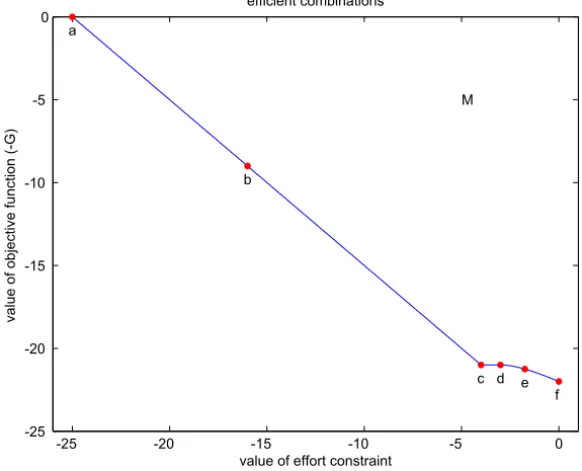
The Figures 1 to 6 show profiles representing gain-optimal combinations. Fig-ure 7 summarizes the development of the gain-optimal combinations and high-lights particular combinations realized by the following profiles. The sum of this graph and the positive orthantR2+would have to be convex if(−G,Eˆ)were
convex-like.
W.l.o.g. gain-optimal combinations will be considered for E = 25 as the shape of(−G,Eˆ)+R2
+remains constant.
Figure 1 shows the unique profile realizing an gain-optimal combination for ˜
E =0. This combination,(0,−25), is denoted byain Figure 7.
Figure 2 depicts a profile representing the gain-optimal combinations for ˜
E = 9. Any feasible profile with −G(p) = −9 is a representative of this combination. In figure 7 it can be found at pointb.
Figure 3 displays the unique profile yielding the gain-optimal combination for ˜
E = 21. Any profile excavating less material from the dark gray in favor of more from the light gray would generate a smaller gain and any profile excavat-ing more of the dark gray area would violate the slope constraint.
As there is no feasible profile generating more thanG(p)=21 with E˜ =22, Figure 4 shows a realization of the gain-optimal combination(−21,−3).
The excavation process along the gain-optimal profiles is continued by ex-tending the latter profile such that as much as possible of the valuable material in layer three is excavated. Figure 5 shows an intermediate state on this excava-tion process.
This procedure continues until the profile which is obtained fulfills the stabil-ity condition as an equalstabil-ity everywhere. The corresponding profile can be seen in Figure 6.
Obviously, the set M which is generated by addition of the first quadrant to this graph is not convex as for example the line connecting the pointscand f cannot be in the resulting setM.
A remedy for the lack of convex-likeness is applying the convex hull operator on the image of the composite mapping. This extends the class of problems for which strong duality can be shown. Recall, that the convex hull of a setK is
the smallest convex set containingK. With the help of this operator, now one is
Figure 1: (a) Figure 2: (b)
Figure 3: (c) Figure 4: (d)
Figure 5: (e) Figure 6: (f)
Theorem 3.1. If the set (−G,Eˆ)(p)with p ∈ P has a supporting tangent at
-25 -20 -15 -10 -5 0 -25 -20 -15 -10 -5 0 efficient combinations
value of effort constraint
va lu e o f o b je ct ive f u n ct io n (-G ) a b
c d e f M
Figure 7 – Development of gain-optimal combinations.
Proof. The main argument of the proof of Theorem 2.1 consist of the fact that
M =(F,g)(Sˆ)+R+×CY
is convex under the additional assumption of convex-likeness of the composite mapping. Then(F(x∗),0)can be separated fromM.
To avoid the convex-likeness of the composite mapping, one has to ensure, that (−G(p∗),0)still can be separated from a convex set containing all combinations (−G,Eˆ)(P). Consider the set
MC =conv
(−G,Eˆ)(P)
+R+×CY.
As a direct sum of two convex sets it is convex as well. By definition, (−G,Eˆ)(p∗) is an element of the convex hull conv
(−G,Eˆ)(P)
and by
optimality one has(−G,Eˆ)(p∗) /∈i nt(MC). Consequently, with
M := MC+R2+
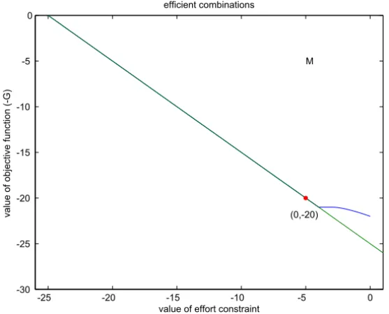
-25 -20 -15 -10 -5 0 -30 -25 -20 -15 -10 -5 0 efficient combinations
value of effort constraint
va lu e o f o b je ct ive f u n ct io n (-G ) (0,-20) M
Figure 8 – Separation of(0,20)by a linear functional.
By Example 1 it will be shown, that the given condition indeed covers a wider class of problems than the convex-like ones.
As one can observe in Figure 7 all convex combinations of the pointscand f for the weightsλ∈(0,1)are not contained in M.
If one applies Theorem 3.1 one can separate the point(−G(p∗),0)from the set M˜ by a linear functional as long as the upper bound on the total effort is E ≤21. In Figure 8 this can be observed forE =20.
In fact, it depends strongly on the effort bound Eˉ whether strong duality can be obtained or not. From this connection one can derive the following corollary for (CFOP). Let p∞denote the globally optimal profile.
Corollary 1. If the global minimum of −G withinP is attained by a profile
p∞∈P that satisfies the capacity constraint of the open pit, i.e.
min
p∈P−G(p)= min
p∈P
ˆ
E(p)≤0
−G(p),
Proof. Obviously,(−G,Eˆ)(p∞)has to be an element on the boundary ofMC.
Hence Theorem 3.1 is applicable.
Thus a characterization of the global minimizer can be obtained if p∞ can
be reached without violating the effort constraint. In the next Corollary, pU
denotes the so calledultimate pitrepresenting the maximal profile in the sense of the lattice structure ofP (see [2, Proposition 3]) which can be reached without
considering any effort constraint or gain optimality.
Corollary 2. If E ≥ E(pU) holds, there is no duality gap between the
primal and the dual problem.
Proof. The global minimizer of the objective has to be attained by the feasible profiles satisfying the capacity constraint because pU is an upper bound for all
profiles in the optimization process. Hence one can apply Corollary 1.
A mining engineer can be expected to define the capacity of the mine large enough to be able to excavate the global minimizer p∞ but not the ultimate
pit pU.
All in all one concludes that the investigation of the gain-optimal profiles is one of the main challenges in the dualization theory for (CFOP). In the opinion of the authors, the approach presented by Matheron [10] provides the best frame-work for this task.
According to Theorem 2.2 the following saddle point property holds for (CFOP) in the case of(−G,Eˆ)being convex-like.
Proposition 3.2 (Saddle Point of the Lagrangian). If the composite mapping (−G,Eˆ)(P)→R×Ris convex-like w.r.t. the product coneR+×R+, p∗is a
solution of (CFOP) if and only if there exist a yˉ ∈ R+ s.t. (p∗,yˉ)is a saddle point of
L(p,y)= −G(p)+ hy,Eˆ(p)i.
4 Full Dual w.r.t. capacity constraint and slope constraint
continuous approach is the possibility to obtain a dual variable for this one and get information about the sensitivity for this constraint.
In the following section an extended problem formulation will be analyzed. In this formulation the stability condition is not longer given implicitly but as an inequality constraint. The problem is given by
min −G(p) s.t. p ∈ ˜P
ˆ
3(p(∙)) ≤0 ˆ
E(p) ≤0
(CFOP′)
where3(ˆ p(∙))=3p(∙)−ω(∙,p(∙))represents the difference of the local slope
of the profile and the value which it is allowed to be at most in a pointwise manner. Moreover,P˜ denotes a special subset of the vector space of
continu-ous functions. In general continucontinu-ous functions do not have to admit a bounded 3p(e.g.,g(x)=x3/2sin(1/x)).
If this quantity is not bounded one is not able to make any assertion on the difference3. Hence one has to pass fromˆ C() to a subset of functions sat-isfying certain regularity conditions. This functions will be in the subspace of Lipschitz continuous functionsLi p()which is dense inC()and guarantees the operator3p(x)at least to be finite for all considered profilespand allx ∈.
The feasible set is now
˜
P≡p ∈Li p()|psatisfies boundary and nonnegativity condition
For the investigation of the duality properties of problem (CFOP′) one has to know about the range space of the constraint mapping. The first component is, as shown above, the space of real numbersR1. For the difference of local Lipschitz constant andωthe following Lemma answers this question.
Lemma 4.1 (range space of the slope constraint).The difference representing the slope constraint
ˆ
3(p(∙))=3p(x)−ω(x,p(x))
is an element of L∞()for any profile p∈ ˜P.
To be able to describe the Lagrange multipliers concerning (CFOP′), the dual space ofL∞()has to be introduced. According to Yosida and Hewitt [12] this
is the space of finitely additive signed measures or shortlybaspace which is a notation introduced in [5, IX.2.15]. Herebais short forbounded additive. The space of the finitely additive signed measure endowed with the norm of total variationkμkvar is a Banach space and will be referred to as (ba(),k ∙ kvar).
To verify that it is indeed a Banach space see e.g., [1, section 4.19]. The space of bounded linear functionals on L∞()can be identified with this space as it can be found in [12, Theorem 2.3].
The ordering cone on the vector space L∞()contains all functions which are not negative almost everywhere, i.e.
CL∞()≡f ∈L∞()|f(x)≥0 for almost allx ∈ . (4)
It is well known that this cone is closed and it’s interior is the set of all essen-tially bounded functions with an essenessen-tially infimum being strictly greater than zero.
The extended problem formulation (CFOP′) is a problem which is equivalent to (P) as well. P˜ ⊂ Li p()is a nonempty subset of a vector space as at least
the initial profile is contained in it. The range space of the constraint mapping (Eˆ,3ˆ p): ˜P →R×L∞()is a totally ordered vector space with ordering cone R+×CL∞(). The feasible setScontains all profiles inP˜ satisfying the capacity
constraint and the slope constraint, i.e. one has
S=p∈ ˜P|(Eˆ,3)(ˆ p)∈ −(R+×CL∞())
This set is nonempty as well as again the initial profile has to be an element of it in the case of E ≥ 0. To determine the dual cone of the range space of the inequality constraint recall the dual space of it.
R+×ba()
The dual cone of the space of essentially bounded functions contains all finitely additive signed measures assigning any measurable subset ofa non negative real number, i.e.
CL∗∞() ≡
HereB()denotes the set of all Borel sets in . The claim will be proven by
contradiction. Letμbe a finitely additive signed measure in the dual cone with μ(A) < 0 for at least one measurable subset A ⊂ . The indicator function χA of this set is an element of the ordering cone of the essentially bounded
functionsCL∞() as it only attains the values 0 and 1. For this function one
obtains
hμ, χAi = Z
χA(x)dμ(x)= Z
A
1dμ(x)=μ(A)≤0
what contradicts the definition of the ordering cone.
As the ordering coneR+×CL∞() is closed one might pass from (CFOP′) to
the equivalent penalized form
min
p∈ ˜P
sup
l ∈R+
μ∈C∗L∞()
−G(p)+ hl,Eˆ(p)i + hμ,3(ˆ p)i. (6)
The corresponding dual problem
max
l∈R+
μ∈C∗L∞()
inf
p∈ ˜P
−G(p)+ hl,Eˆ(p)i + hμ,3(ˆ p)i (7)
gives at least a lower bound on the extremal value of problem (CFOP′). More-over, under certain additional requirements, it is possible to show the validity of strong duality what is proven by the following proposition.
Proposition 4.1 (Duality and the Extended Problem). If the composite map-ping(−G, (Eˆ,3))(ˆ P˜)is convex-like w.r.t. the product coneR+×CY and (GSC)
is satisfied the Theorem2.1is applicable.
Hence the dual problem(7)is solvable and the extremal values of both prob-lems coincide.
Proof. The proof is analogous to Theorem 2.1.
In the setting of (CFOP′) the existence of a profile in the interior points of the ordering cone is a non trivial property. As the product coneCY =R+×CL∞()
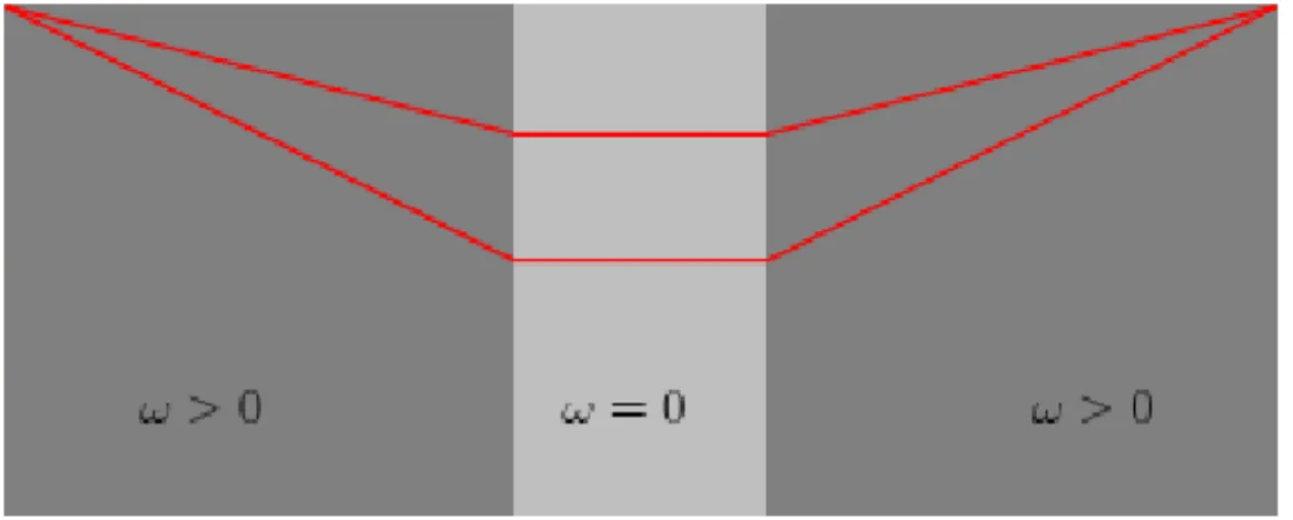
an element of the interior points of both original cones. As the existence of a profilepwithEˆ(p)∈i nt(R+)is ensured easily as seen in the preceding section, this is not clear for the slope condition. For example consider a volume with a vertical part where no slope is possible for a profile. A two dimensional sketch of this scenario can be found in Figure 9.
Figure 9 – Volume with vertical inclusion.
Here one can observe immediately, thatanyprofile phas to satisfy
ˆ
3(p)(x)=0
for allx withω(x,∙)=0. In this case there cannot exist a profile in the interior of the negative ordering cone of−CL∞() as these elements has to be strictly
smaller than zero almost everywhere.
A possible remedy is to assume the initial profile p0to be an element of the feasible profiles which does strictly fulfill the slope condition anywhere accord-ing to [2, Proposition 2.3]. Then a profile in the interior of the product cone would be guaranteed.
According to Theorem 2.2 the following characterization of solutions for the extended problem formulation (CFOP′) in the case of(−G, (Eˆ,3))ˆ being convex-like can be given.
Proposition 4.2 (Saddle Point property). If the composite mapping
(−G,Eˆ,3)(ˆ P˜)→R×R×L∞()
is convex-like w.r.t. the product cone R+×R+×CL∞(), p∗ is a solution of
a saddle point of
L(p,y1,y2)= −G(p)+ hy1,Eˆ(p)i + hy2,3(ˆ p)i. 5 Conclusions
We were able to apply the duality theory for convex-like optimization prob-lems to the stationary problem (CFOP) and the extended problem formulation (CFOP′). Correspondingly the existence of Lagrange multipliers for the effort constraint and also the slope constraint was proven.
Unfortunately this Lagrange multiplier in general only is a measure. This lack of functional regularity provides a challenge for numerical methods. Typical remedies are known, e.g. from PDE constraint optimization and can be distin-guished into two main concepts. The first is to consider an a priori discretized problem as in [3]. The second one is to regularize the constraint yielding a Lagrange multiplier that is a function and can thus be conveniently represented and manipulated numerically.
Suitable numerical schemes are currently under investigation.
REFERENCES
[1] H.W. Alt,Lineare Funktionalanalysis: Eine anwendungsorientierte Einfuhrung.
Springer Verlag, (2006).
[2] F. Alvarez, J. Amaya, A. Griewank and N. Strogies, A continuous framework for open pit mine planning. to appear in Mathematical Methods for Operations Research.
[3] M. Bergounioux and K. Kunisch,Primal-dual strategy for state-constrained opti-mal control problems.Computational Optimization and Applications,22(2002), 193–224.
[4] L. Caccetta and L.M. Giannini, An application of discrete mathematics in the design of an open pit mine.Discrete Applied Mathematics,21(1988), 1–19.
[5] N. Dunford and J.T. Schwartz,Linear operators, part I.Interscience, New York, (1958).
[7] K. Ito and K. Kunisch,Lagrange Multiplier Approach to Variational Problems and Applications.SIAM, (2008).
[8] J. Jahn, Introduction to the theory of nonlinear optimization.Springer Verlag, (2007).
[9] V. Jeyakumar,Convexlike alternative theorems and mathematical programming.
Optimization,16(1985), 643–652.
[10] G. Matheron,Le paramétrage des contours optimaux.Technique notes,401, 19– 54.
[11] R.T. Rockafellar and R.J.-B. Wets,Variational analysis.Springer Verlag, (1998).