Copyright © 2011 SBMAC ISSN 0101-8205
www.scielo.br/cam
Stochastic Newton-like methods for computing
equilibria in general equilibrium models
NATAŠA KREJI ´C1∗, ZORANA LUŽANIN1∗ and ZORAN OVCIN2 1Department of Mathematics and Informatics, Faculty of Science
University of Novi Sad, Trg Dositeja Obradovi´ca 4, 21000 Novi Sad, Serbia
2Faculty of Technical Sciences, University of Novi Sad, Trg Dositeja Obradovi´ca 6
21000 Novi Sad, Serbia
E-mails: natasak@uns.ac.rs / zorana@dmi.uns.ac.rs / zovcin@uns.ac.rs
Abstract. Calculating an equilibrium point in general equilibrium models in many cases reduces to solving a nonlinear system of equations. Taking model parameter values as random variables with a known distribution increases the level of information provided by the model but makes computation of equilibrium points even more challenging. We propose a computationally efficient procedure based on application of the fixed Newton method for a sequence of equilib-rium problems generated by simulation of parameters values. The convergence conditions of the method are derived. The numerical results presented are obtained using the neoclassic exchange model and the spatial price equilibrium model. The results show a clear difference in the quality of information obtained by solving a sequence of problems if compared with the single equilibrium problem. At the same time the proposed numerical procedure is affordable.
Mathematical subject classification: 65H10, 91B50.
Key words:nonlinear system of equations, Newton-like method, general equilibrium model.
1 Introduction
The problem we consider in this paper is
F(x,W)=0, (1)
#CAM-319/10. Received: 15/VIII/10. Accepted: 05/I/11.
wherex ∈Rnis an unknown vector,W is am−dimensional vector of parame-ters andF :Rn →Rn.
The most simple case of this type of problems arises when W ∈ Rm is con-stant. Many economic models can be written in the form of (1) withW being a vector of parameters that are estimated. Estimation of the parameter values based on real data is a nontrivial task given thatWis most likely a random vec-tor. As F is often highly nonlinear andn can be large, solving (1) becomes a challenging issue soWis often replaced by a constant real valued vector, say by the expected value. Such modeling simplification makes solving (1) easier but also introduces additional uncertainty into the model. An important part of the information available from the real data might be lost with the constant value parameters approach and hence the model properties might deteriorate. There-fore the question of finding a computationally affordable procedure for solving (1) withW being more general than just a constant vector naturally arises.
Let us assume that W in (1) is estimated in such a way that its probability distribution is known. So W is a random vector on some probability space
(,F,P). This kind of parameter estimation provides significantly larger
amount of information than constant value and thus implies better properties of the model. In that case (1) becomes a stochastic problem and its solution can be a random variable. Analytical solution of (1) is not available in general and thus an affordable numerical procedure is of great interest.
Solving stochastic nonlinear systems of equations numerically is a difficult problem. A number of numerical procedures is suggested and analyzed in liter-ature if the parameter vectorWis a constant, [10, 6, 7]. The proposed numerical procedures are in fact designed for solving the deterministic nonlinear problems of the form (1) and they are mainly based on the interior-point or homotopy methods. In this paper we propose a different approach aiming to preserve as much information about the vectorW as possible but keeping the computational cost at a reasonable level. IfWis a random vector with known distribution then for a given sample{w1, . . . , wN}one could solve the sequence of problems
F(x, wi)=0, i =1, . . . ,N (2)
getting a sequence of solutions (x∗1, . . . ,x∗N) ∈ Rn×N.If N is large enough then (x∗1, . . . ,x∗N
random vector x∗ which is a solution of (1). However solving the sequence of nonlinear systems (2) for large values of N might be computationally unaf-fordable. Therefore we are proposing a numerical procedure based on the fixed Newton idea that generates a sequence of approximate solutions of (2) at an affordable cost and thus provides significantly more information that a solution of (1) for a constant value (i.e. the expected value) of the vectorW.
Section 2 of this paper contains the algorithm we are proposing and its con-vergence analysis. Two equilibrium models of the form (1) are described in Section 3 and the numerical results are presented in Section 4.
2 The Algorithm
Let us assume that W is a random vector with a known distribution and the sample(w1, . . . , wN) is drawn. We are interested in solving the sequence of
problems
F(x, wj)=0, j =1, . . . ,N,
and thus obtaining the sequence of optimal solutions
(x∗1, . . . ,x∗N)∈Rn×N.
The final goal is to obtain an approximation ofx∗,which is a random variable that solves (1). So forN large enough we can use the sequence(x∗1, . . . ,x∗N) to estimate the distribution of each component ofx∗.
The problem (1) is considered under a set of standard assumptions. Let D⊂Rnsuch that the following assumptions are satisfied.
(A1) For allw∈there existsxw∗∈ Dsuch thatF(xw∗, w)=0.
(A2) For allw∈the Jacobian matrix F′(xw∗, w)is nonsingular.
(A3) For allx,y ∈ Dandw∈there existsγ >0 such that
||F′(x, w)−F′(y, w)|| ≤γ||x−y||
(A4) For allwi, wj ∈andx ∈ Dthere existsγW >0 such that
One obvious possibility is to use the Newton method to solve each of the systems (2). The Newton method is a reliable choice given that it yields quadratic convergence for a good initial approximation. So givenxi,0the sequence
F′(xi,k, wi)si,k = −F(xi,k, wi), xi,k+1=xi,k+si,k, k =1,2, . . . (3)
will converge to the solutionxi∗if F(x, wi)satisfies the standard assumptions
A1-A3. However such procedure would be quite expensive for large N if the dimensionnof the problems (2) is even a modest number. On the other hand the Jacobian matricesF′(xi,k, wi)could be expected to have very similar structure for different sample realizations wi.Therefore a numerical procedure should
take advantage of such similarity. A natural way to employ the favorable prop-erties of the sequence of problems we are solving would be consider the proce-dure based on the fixed Newton approach. The fixed Newton method calculates the Jacobian only once and proceeds with iterations using the initial Jacobian during the whole process. The method is convergent if the initial approxima-tion is close enough to the soluapproxima-tion of the considered nonlinear system. So we will consider the following algorithm for solving (2).
Algorithm FNM
Step 0: Letx0∈Rnand(w1, . . . , wN)be given. Calculate the mean value
ˉ
w=
N
X
i=1
wi/N
and solve F(x,w)ˉ = 0 by the Newton method. Denote the solution by xwˉ and define A=F′(xwˉ,w).ˉ
Step 1: Fori =1, . . . ,N
Step 1i: Setxi,0=xwˉ
Step 2i: Repeat until convergence
Remark. The suggested matrix A=F′(xwˉ,w)ˉ is one possible choice for the constant matrix used in Step 2i. The main computational burden in (3) comes from the calculation of the Jacobian at each iteration and for each sample re-alizationwi, followed by solving the corresponding linear systems that define
the iteration increments si,k. Therefore the main advantage of the suggested procedure is that all steps are obtained by solving a system of linear equation with the same matrix A. Naturally Ashould be a reasonably good approxima-tion of the true Jacobians at all iteraapproxima-tions. Furthermore Acan be factored only once and used in each Step 2i thus decreasing the linear algebra costs signif-icantly. So calculating A with the sample mean wˉ appears natural given that such Ashould be reasonably close to F′(x, wi)for allwi and x close toxi∗.
But there are several other possibilities, for example A = F′(x0, wj),with j being an arbitrary number 1 ≤ j ≤ N.The numerical testing we performed
did not indicate that the algorithm exhibits large differences depending on the choice ofwˉ or anywj when defining A.More details are reported in Section 4. The algorithm above will generate the sequence (x1∗, . . . ,xN∗)if Step 2i is
well defined i.e. if every single iterative procedure fori = 1, . . . ,N ends up with somexi,k that satisfies the convergence conditions and could be taken as xi∗ in Step 3i. One of the advantages of the above algorithm is that it could be easily used in parallel environment [2].
We will prove that the standard assumptions (A1)-(A4) imply that Step 2i is well defined. The convergence theorem presented below is based on the Banach contraction principle. The convergence condition might be seen as a general-ization of two neighbourhod theorem as it consists of an inequality connecting the distance between the initial point and the solution and the variance of the model parametersW.Such condition might seem rather strong as common in
local convergence statements. But the numerical results given in Section 4 will demonstrate the effectiveness of the algorithm despite the strong convergence condition.
Let us denote B = B(x, δ) = {y ∈ Rn : kx − yk ≤ δ}.Assuming that
Assumptions A1-A3 are satisfied one can easily see that the Newton method for solving F(x,w)ˉ = 0 is locally convergent i.e. there exists δ1 > 0 such that for x0 ∈ B(xwˉ∗, δ
sequence. Letxwˉ be the value obtained aftersiterations of the Newton method in Step 0 and let s be large enough such that xwˉ is close enough to xwˉ∗. Then the matrix F′(xwˉ,w)ˉ is nonsingular and there exists M > 0 such that ||F′(xwˉ,w)ˉ −1|| = M. The convergence of FNM Algorithm is stated in the
theorem below.
Theorem 1. Let F satisfy assumptions A1-A4. If for εW = diam() and M = ||F′(xwˉ,w)ˉ −1|| there existsδ > 0such that α = M(γ δ+γ
WεW) < 1 and||F′(xwˉ,w)ˉ −1F(xwˉ, wi)|| ≤ δ(1−α) then for everywi ∈ sequence {xwi,k}∞k=0, i = 1,2, . . . ,N defined by Step 1 of Algorithm FNM converges linearly to solution F(x, wi)=0.
Proof. LetG(x)=x −F′(xwˉ,w)ˉ −1F(x, wi). Then, forx ∈B ||G′(x)|| = ||I −F′(xwˉ,w)ˉ −1F′(x, wi)|| ≤ ||F′(xwˉ,w)ˉ −1||
×(||F′(xwˉ,w)ˉ −F′(x,w)ˉ || + ||F′(x,w)ˉ −F′(x, wi)||) ≤ M(γ||xwˉ −x|| +γ
W|| ˉw−wi||)≤ M(γ δ+γWεW) = α <1
From the mean-value theorem we obtain
||G(x)−G(y)|| ≤ sup t∈[0,1]
||G′(x+t(y−x))||∙||x−y|| ≤α||x−y||, ∀x,y∈B.
Therefore,Gis contraction onB.Further more
||G(x)−xwˉ|| ≤ ||G(x)−G(xwˉ)|| + ||G(xwˉ)−xwˉ|| ≤αδ+δ(1−α)=δ
and G maps B into itself. Therefore the contraction mapping theorem
ap-plies and there exists a unique fixed point in B and that point is the solution
ofF(x, wi)=0 inB.
3 Equilibrium models
Neoclassical exchange economy
formalized by Arrow and Debreu, [7, 11] and since then extensively analyzed in the literature, [11, 3, 9]. One survey of the general equilibrium models is presented in [6]. The most common approaches for solving equilibrium prob-lems include simplex methods based on the constructive proof of the Brouwer fixed point theorem, tâtonnement approach, Newton method, Smale’s method, interior-point method (see [6] and references therein). Homotopy method is analyzed in [4].
LetRn+ be the set of nonnegative real numbers. The model we will consider assumes that there are n commodities in X ⊂ Rn+ and m economic agents. Each agent has a utility function uj, and an initial endowment ωj for j = 1, . . . ,m.Therefore each agent has the budget π ∙ωj where π ∈ Rn+ is the price vector of commodities. The choice of utility function is defining the model. We will consider the following three possibilities.
• Cobb-Douglas:u(x)=xa1
1 ∙ ∙ ∙xnan, n
X
i=1
ai =1, ai ≥0
• fixed proportional:u(x)=min
x1 a1,∙ ∙ ∙,
xn an
, ai >0
• CES:u(x)= n
X
i=1
ai1/bxi(b−1)/b
!b/(b−1)
, ai >0, b≤1
In any of these utility functions the set of parameters a1, . . . ,an,b has to be estimated. The models considered in [6] assume that these values are constant, while we consider a more general case in which these parameters are random variables with known distribution.
All agents are profit maximizers, the goal is to maximize the chosen utility function for each agent i.e. to determine
xj(π )=arg max πx≤π ωju
j(x), j =1, . . . ,m.
For the considered utility functions we have the following maximizers
• Cobb-Douglas demand function: xij(π )= π∙ω j
πi
• fixed proportions demand function: xij(π )= π∙ω j
π∙aj a j
i, i =1,2, . . . ,n
• CES demand function: xij(π )= π ∙ωj
πibj
n
X
k=1
πk1−bjakj
aij, i =1,2, . . . ,n.
If the excess demand function is defined as
ξ(π )= m
X
j=1
xj(π )− m
X
j=1
ωj,
then any strictly positiveπ∗such that
ξ(π∗)=0 (4)
is an equilibrium price.
Spatial price equilibrium model
The class of market equilibrium problems where supply, demand and trans-portation cost functions are nonlinear and separable is considered in [10] and the references cited therein. The distinguishing characteristic of spatial price equilibrium models lies in their recognition of the importance of space and transportation costs associated with shipping a commodity from a supply market to a demand market. These models are perfectly competitive partial equilib-rium models. The model we consider assumes that there are many producers and consumers involved in the production and consumption, respectively, of one or more commodities.
We will use the following notation.
• Yi – total supply (output) at origin (market)i ∈ I = {1, . . . ,m}
• Zi – total demand (input) at destination (market) j∈ J = {1, . . . ,n}
• xi j – quantity shipped (traded) from origini∈ I to destination j ∈ J
• Ij(Zj)– inverse demand function at destination j
• ci j(xi j)– transportation (transaction) cost between origini and destina-tion j
The equilibrium can be described as a triple{(Yi)i∈I, (Zj)j∈J, (xi j)i∈I,j∈J}that solves the system of equalities and inequalities
Si(Yi)+ci j(xi j)
= Ij(Zj), if xi j >0
≥ Ij(Zj), if xi j =0
Yi =X j∈J
xi j, ∀i∈ I
Zj =
X
i∈I
xi j, ∀j ∈ J
xi j ≥0, ∀i, j ∈ I ×J
(5)
The model is developed assuming that the following assumptions hold.
M1 The supply, demand and transportation cost functions are nonnegative C1(R+) functions. The supply and transportation functions are nonde-creasing while the demand price is noninnonde-creasing.
M2
lim Yi→∞
Si(Yi)= +∞, lim
Zi→∞
Ij(Zj)=0
If M1-M2 hold then the equilibrium conditions (5) are the KKT conditions for the minimization problem
min
x≥0G(x)=
X
i∈I
Z Pj∈Jxi j
0
S(t)dt+X i∈I
X
j∈J
Z xi j
0
ci j(t)dt−X j∈J
Z Pi∈Ixi j
0
I(t)dt
Supply, demand and transportation costs are model parameters that need to be estimated whilexi j are the unknowns we want to compute at the equilibrium.
If a shipping quantity xi j is zero, the corresponding inequality in (5) can be strict. As in ([10]) we can assume the strict complementarity hypothesis:
in the solution (x∗,Y∗,Z∗). Otherwise we have degeneracy. Most common situation for degeneracy is when the transportation cost functions ci j(xi j)are
constant. Under the strict complementarity assumption, we can apply some strategy for determining set of indicesPwith nonzero shipping quantities. That
gives us system of equations from (5) for (i, j) ∈ P. However, in our
com-putations it was not needed, as the problems we considered had allxi j positive (P =I ×J).
Denoting by x the components xi j,i ∈ I,j ∈ J and by W all model para-meters we can write the conditions (5) asF(x,W)=0.
4 Numerical results
In a Neoclassical exchange economy we find the equilibrium price by solving the system (4) for a price vectorπ∗. As a consequence of the homogeneity of degree zero of the demand and supply functions in the prices, without loss of generality, we can define prices and look for the solution on the positive simplex
1+=
(
π ∈Rn+
n
X
i=1
πi =1
)
.
In numerical calculations we shall substitute the last equation in the system (4) with the equationPn
i=1πi =1. Statistics
In order to see the effects of our Algorithm, we perform several calculations with different parameter values. In all examples the values of parameters are generated as pseudo-random numbers having normal or uniform distribution with given deviation centered about the value that occurs in the standard testing problems. The first phase of the algorithm yields xwˉ where wˉ is the sample mean. Given that all mappings are nonlinear that point is just an approximation to the solution mean. Although this approximation was relatively close to the sample mean in all tested examples Step 1 of FNM algorithm further improves the approximate solution x∗i for each sample wi and thus generates a sample
For each solution some descriptive statistics are presented. We also perform a statistical test to verify or reject the hypothesis that the solution sample is normally distributed as the parameters samples. The test for normality we use is the Anderson-Darling test ([1]) with significance levelα=5%. The Anderson-Darling statistics is
A2= −1 N
( N X
i=1
(2i−1)lnzi +ln(1−zN+1−i)
)
−N,
whereN is the sample size, andzi is thei-th value in the sorted sample. We use the modified Anderson-Darling statistics
A2m = A2
1+ 0.75
N +
2.25
N2
,
whose critical value for significance levelα =0.05 is 0.752, and critical value
forα=0.01 is 1.035.
The values for kurtosis and skewness of a component of the solution sample
π∗i,i=1, . . . ,Nare presented in the Figures. These values describe the shape of the probability density function of the sample component distribution. The formulas for skewness and kurtosis are given by
β12=μ23/μ23, β2=μ4/μ22 respectively, where
μk = 1 N
N
X
i=1
(xi −m1)k , m1= 1 N
N
X
i=1
(xi) .
Kurtosis is 0 and skewness is 3 for normal distribution.
The values ofβ12,β2, histogram, statistical momentsm1andμk, the Anderson-Darling statistics and other descriptive statistics data are examples of valuable information on the behavior of the equilibrium prices under Gaussian noise i.e. under the assumption of normal distribution of parameter values.
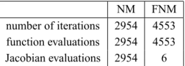
Example 1
NM FNM number of iterations 2954 4553 function evaluations 2954 4553 Jacobian evaluations 2954 6
Table 1 – Solving equilibrium for Neoclassical exchange economy (6), (8) with 2 goods and 2 agents, sample ofN=500 parameter values.
function is the Cobb-Douglas functionu1(π )=πa
1 1
1 π 1−a11
2 . The second agents’ utility function is the fixed proportions utility functionu2(π )=min
n
π1
a21, π2
a22
o
. The excess demand functions in this case are the following
ξ1(π )=a11
3π1+π2
π1
+a12
π1+2π2 a12π1+a22π2
−4 (6)
ξ2(π )=(1−a11)
3π1+π2
π2
+a22 π1+2π2 a21π1+a12π2
−3. (7)
In our calculations we modify the system (4) intoξ (π )ˉ =0 by substituting (7) with
ξ2(π )=π1+π2−1. (8)
The initial value for the Newton method (NM) is taken asπ0=(0.1,0.9)for all sample values and the exit criterion for both the Newton method and the fixed Newton method (FNM)|| ˉξ||< ǫ =10−6.
Taking parametersa11 = 0.4,a12 = 2, a22 = 3, we obtain the solution π∗ =
(0.2087,0.7913)by the Newton method in 6 iterations.
Next, we make samples of N = 500 values for parameters from normal dis-tribution: a11 : N(0.4,0.05), a12 : N(2.0,0.05), a22 : N(3.0,0.05). Let W denotes the triple of parametersW =(a11,a12,a22)andwi,i =1, . . . ,N be the set of the sample values.
We perform both methods (Newton’s and FNM) for the parameter sample values obtaining the sample of solutionsπ∗i,i=1, . . . ,N.
The average number of iterations in each of 500 problems is 5.91 for NM and 9.11 for FNM but the CPU time clearly demonstrate the advantage of FNM approach as it is 0.156 for NM and 0.098 for FNM.
The histogram and descriptive statistics of the solution sample for both com-ponentsπ∗
1 andπ2∗are shown in Figure 1. We get the same values ofπ1∗andπ2∗ as they are not independent (π1+π2=1).
Problem (4) is a continuous mapping from the parameter set into the solution set. Thus the obtained solution sequence is a sample from a random variable. If it is a sample from a random variable, from the histogram we could say that the probability distribution of the underlying distribution is bell shaped, slightly slanted (β12 = 0.1090, should be zero for symmetric random variable
like normal distribution). The kurtosis parameter of the sample isβ2 =2.9419, near 3, the kurtosis of normal distribution.
However, test for normality of the sample gives the value for adjusted AD statisticsA2m =1.3263 that is larger than the critical value. So we reject the null
hypothesis of the normality of the solution sample (P <0.0019).
This tells us that if one wants to estimate confidence intervals for sample values, knowing the distribution of parameters, the limiting values of the confi-dence intervals for normal distribution cannot be used.
Example 2
We consider a Neoclassical exchange economy withn = 3 goods andm = 4 agents with the CES utility function. The Excess demand functions are
ξj(π )= 4
X
i=1
" P3
k=1ωikπk
πbjiP3
k=1αikπ 1−bi
k
αij−ωij
#
, for j =1,2,3. (9)
In this Example, parameters and initial endowments are given in the follow-ing matrices
α :=α0=
0.1 0.7 0.2
0.1 0.4 0.5
0.2 0.3 0.5
0.9 0.05 0.05
, ω:=ω0=
2 1 1 1 2 0 2 0 3 1 1 2
, b :=b0 =
0.5
0.5
0.5
0.5
0.1 0.15 0.2 0.25 0.3 0.35 -20
0 20 40 60 80 100
N = 500, m1 = 0.2095, std = sqrt(mu2) = 0.0390, beta12 = 0.1090, beta2 = 2.9419
Anderson-Darling statistic: 1.3243 Anderson-Darling adjusted statistic: 1.3263
Probability associated to the Anderson-Darling statistic = 0.0019 With a given significance alpha = 0.050
The sampled population is not normally distributed.
(a)
0.65 0.7 0.75 0.8 0.85 0.9 0.95 1
-20 0 20 40 60 80 100
N = 500, m1 = 0.7905, std = sqrt(mu2) = 0.0390, beta12 = 0.1090, beta2 = 2.9419
Anderson-Darling statistic: 1.3243 Anderson-Darling adjusted statistic: 1.3263
Probability associated to the Anderson-Darling statistic = 0.0019 With a given significance alpha = 0.050
The sampled population is not normally distributed.
(b)
and i-th row of a matrix representsi-th agents’ data. In our notation, the elements in thei-th row and j-th column of matricesαandωareαij andωij. We getξˉ
by substituting the last equation in (4) with
ξ3(π )=π1+π2+π3−1. (10)
Given the initial value π0 = (0.4,0.2,0.4), the Newton method with exit criterion || ˉξ|| < ǫ = 10−6 in 7 iterations gives the solution π∗ = (0.2441,
0.5566,0.1993).
The sample used in this Example is obtained by perturbing components of parameterb: bi,i =1,2,3,4 with N =500 normally distributed values, bi :
N(0.5,0.1),i =1,2,3,4.
Like in Example 1, the total number of iterations, number of function evalua-tions and Jacobian evaluaevalua-tions for both NM and FNM are given in Table 2. The average numbers of iterations are 6.60 and 9.16 for NM and FNM respectively but the corresponding CPU times are 1.267 and 0.820.
NM FNM
number of iterations 3301 4581 function evaluations 3301 4581 Jacobian evaluations 3301 7
Table 2 – Solving equilibrium for Neoclassical exchange economy (4) with (9), (10), CES utility function, with 3 goods and 4 agents, sample ofN=500 parameter values.
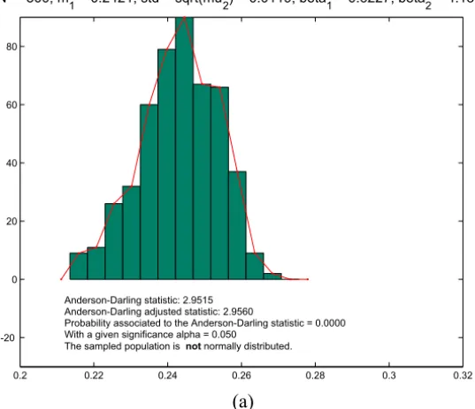
Descriptive statistics of the solution sample are given in Figure 2.
We can easily see from the histogram that the sample is asymmetric (β12>0.6)
and the kurtosis is far from 3, the kurtosis of normal distribution. Even more, AD test tells us the underlying distribution certainly (P <10−5) is not normal. This should be taken in account if confidence intervals for equilibrium prices are sought.
Example 3
0.2 0.22 0.24 0.26 0.28 0.3 0.32 -20
0 20 40 60 80
N = 500, m1 = 0.2421, std = sqrt(mu2) = 0.0119, beta12 = 0.6227, beta2 = 4.1814
Anderson-Darling statistic: 2.9515 Anderson-Darling adjusted statistic: 2.9560
Probability associated to the Anderson-Darling statistic = 0.0000 With a given significance alpha = 0.050
The sampled population is not normally distributed.
(a)
0.45 0.5 0.55 0.6 0.65 0.7
-20 0 20 40 60 80 100
N = 500, m1 = 0.5639, std = sqrt(mu2) = 0.0403, beta12 = 0.8592, beta2 = 4.5633
Anderson-Darling statistic: 4.0471 Anderson-Darling adjusted statistic: 4.0532
Probability associated to the Anderson-Darling statistic = 0.0000 With a given significance alpha = 0.050
The sampled population is not normally distributed.
(b)
0.1 0.15 0.2 0.25 0.3 0.35 -20
0 20 40 60 80 100 N = 500, m
1 = 0.1939, std = sqrt(mu2) = 0.0284, beta1
2 = 0.9710, beta
2 = 4.7381
Anderson-Darling statistic: 4.5708 Anderson-Darling adjusted statistic: 4.5777
Probability associated to the Anderson-Darling statistic = 0.0000 With a given significance alpha = 0.050
The sampled population is not normally distributed.
(c)
Figure 2 (continuation) – Histogram and descriptive statistics of sample of solutionsπ3∗ (c) for sample ofN =500 parameter values for (4) with (9), (10).
Numerical tests are performed assuming that the supply and demand func-tions are
Si(Yi)=ui+
Yi
vi
2
,
Ij(Zj)= 1
θj ln
2000
Zj
,
and the cost functions is linear,
ci j(xi j)=γi jxi j .
Parametersui,vj,θj andγi j belong to the intervals[3,5],[15,20],[0.1,0.5], [5,10]respectively.
The initial value for the Newton method for all sample values isx0=
"
20 20 20 20
#
For the following values of the parameters
u= [4.00,4.00]T, v= [17.50,17.50]T,
θ = [0.30,0.30]T, γ =
"
7.50 7.50
7.50 7.50
#
,
the solution by the Newton method isx∗=
"
2.182 2.182
2.182 2.182
#
,and it is obtained
in 4 iterations.
Using a sample of N = 500 random values for independent components of
v: v1andv2, both normally distributedv1,2:N(17.5,1)and other parameters as above, we solved the equilibrium with the Newton method. After that, as in Example 1 we used the fixed Newton method, with the Jacobian and starting point obtained from the Newton method computed with the mean of parameter sample. The number of calculations is given in Table 3.
NM FNM
number of iterations 5465 3227 function evaluations 5465 3227 Jacobian evaluations 5465 4
Table 3 – Solving SPAT equilibrium (5), with 2 origins and 2 destinations, sample ofN =500 parameter values.
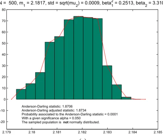
The average numbers of iterations are 10.93 and 6.45 for NM and FNM re-spectively with the corresponding CPU times 1.272 and 0.289. The descriptive statistics of the solution sample is given in Figure 3.
In two out of four cases for the solution sample the null hypothesis is not re-jected. In these cases, an even larger sample is needed to reach the real properties of the solution and in these cases FNM algorithm will be even more efficient.
CPU time and larger dimensions
2.179 2.18 2.181 2.182 2.183 2.184 2.185 -20
-10 0 10 20 30 40 50 60 70 80
N = 500, m1 = 2.1817, std = sqrt(mu2) = 0.0009, beta12 = 0.2513, beta2 = 3.3100
Anderson-Darling statistic: 1.8706 Anderson-Darling adjusted statistic: 1.8734
Probability associated to the Anderson-Darling statistic = 0.0001 With a given significance alpha = 0.050
The sampled population is not normally distributed.
(a)
2.179 2.18 2.181 2.182 2.183 2.184 2.185 -20
-10 0 10 20 30 40 50 60 70 80
N = 500, m1 = 2.1817, std = sqrt(mu2) = 0.0009, beta12 = 0.2513, beta2 = 2.9916
Anderson-Darling statistic: 1.8706 Anderson-Darling adjusted statistic: 1.8734
Probability associated to the Anderson-Darling statistic = 0.0001 With a given significance alpha = 0.050
The sampled population is not normally distributed.
(b)
2.179 2.18 2.181 2.182 2.183 2.184 2.185 -20
-10 0 10 20 30 40 50 60 70 80 N = 500, m
1 = 2.1817, std = sqrt(mu2) = 0.0009, beta1
2 = 0.0803, beta
2 = 2.6652
Anderson-Darling statistic: 0.6576 Anderson-Darling adjusted statistic: 0.6586
Probability associated to the Anderson-Darling statistic = 0.0856 With a given significance alpha = 0.050
The sampled population is normally distributed.
(c)
2.179 2.18 2.181 2.182 2.183 2.184 2.185 -20
-10 0 10 20 30 40 50 60 70 80 N = 500, m
1 = 2.1817, std = sqrt(mu2) = 0.0009, beta1
2 = 0.0803, beta
2 = 2.7725
Anderson-Darling statistic: 0.6576 Anderson-Darling adjusted statistic: 0.6586
Probability associated to the Anderson-Darling statistic = 0.0856 With a given significance alpha = 0.050
The sampled population is normally distributed.
(d)
method are even more evident. To support this claim we tested Example 2 and Example 3 for different values of m and n. Thus for Example 2 we gener-ate the matrixα0 using random numbers scaled to row sums equal to 1, with
w0=2+U(0,1), b= [0.9;0.9;. . .;0.9]. HereU(0,1)denotes independent random numbers with uniform distribution on [0,1]. The tested sample size is 500 again and the results (the total number of iterations and the total CPU1 time) are reported in Table 4 for NM and FNM method.
NM iter NM CPU FNM iter FNM CPU
m=4,n =3 2134 0.773 3156 0.555
m=8,n =6 2893 1.383 3200 0.606
m=16,n=12 3072 3.554 3949 0.959
m=32,n=24 2514 14.592 4144 1.988
Table 4 – Example 2.
For Example 3 parameters wereui =4,vj =17.5+0.5∙N(0,1),θj =0.3 andγi j =7.5 for alliand j. N(0,1)denotes independent normally distributed values with mean 0 and standard deviation 1. The initial value was
x0=
20 ∙ ∙ ∙ 20
..
. . .. ...
20 ∙ ∙ ∙ 20
,
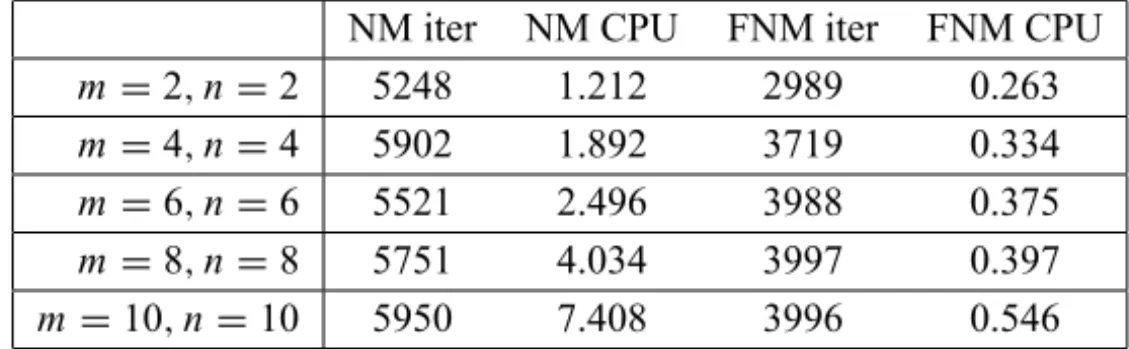
the exit criterion was||F|| < ǫ = 10−6. The results are given in Table 5 – the total number of iteration and the total CPU time in seconds.
NM iter NM CPU FNM iter FNM CPU
m=2,n=2 5248 1.212 2989 0.263
m=4,n =4 5902 1.892 3719 0.334
m=6,n =6 5521 2.496 3988 0.375
m=8,n =8 5751 4.034 3997 0.397
m=10,n=10 5950 7.408 3996 0.546
Table 5 – Example 3.
Conclusion
Equilibrium problems are often formulated as systems of nonlinear equations that depend on parameters. Significantly more information on equilibrium point can be obtained by simulation and solving a sequence of nonlinear systems rather than by solving a single nonlinear system with constant parameter values. We introduce a perturbation of model parameters taking their values from a given distribution sample. For each sample value we solve the corresponding system of nonlinear equations using the same starting point and applying Fixed Newton method. Thus we obtain the sample of solutions for each problem using a relatively cheap procedure. The sample of solutions yields better description of the observed system. For example the presented descriptive statistics show that the assumption of Gaussian distribution of the solution due to the Gaussian distribution of parameters is not guaranteed.
The question of confidence interval formulas for equilibrium prices is still open and it should be investigated from problem to problem. The stochastic simulations (Monte-Carlo) could give more information. If tests find the under-lying distribution was normal, one could use well known formulas for confi-dence intervals for normal distribution. However, the algorithm proposed in this paper can give easier access to larger solution sample.
Solving many nonlinear systems requires a lot of CPU power which is usually limited. In our examples we showed that using similarities within sample data, an affordable procedure can be implemented. In Example 1 and 2 the total number of function calculations has risen following the rise of the number of iterations, but the number of expensive Jacobian calculations was almost zeroed. In Example 3 even the number of iterations lowered. In order to demonstrate the effectiveness of the proposed algorithm we included some tests with larger dimension problems. The number of iterations in these case is in line with small dimensional cases but the CPU time definitely favors the use of FNM method instead of NM method.
REFERENCES
[1] T.W. Anderson and D.A. Darling,Asymptotic Theory of Certain “Goodness of Fit” Criteria Based on Stochastic Processes.The Annals of Mathematical Statistics,
23(2) (1952), 193–212.
[2] J. Arnal, H. Migallón, V. Migallón and J. Penadés, Parallel Newton Iterative Methods Based on Incomplete LU Factorizations for Solving Nonlinear Systems. Lecture Notes in Computer Science,3402(2005), 716–729.
[3] A. De la Fuente, Mathematical Methods and Models for Economists. Cambridge University Press (2000).
[4] B.C. Eaves and K. Schmedders, General equilibrium models and homotopy methods.Journal of Economics & Control,23(1999), 1249–1279.
[5] M.B.M. Elgindi, On the application of Newtonâs and chord methods to bifurca-tion problems.Internat. J. Math. & Math. Sci.,17(1) (1994), 147–154.
[6] M. Esteban-Bravo, Computing equilibria in general equilibrium models via interior-point methods.Computational Economics,23(2004), 147–171.
[7] M. Esteban-Bravo, An interior-point algorithm for computing equilibria in economies with incomplete asset markets.Journal of Economic Dynamics and Control,32(3) (2008), 677–694.
[8] J. Focke, A Simplified Newton Method for Computing the Factor Loadings in Maximum Likelihood Factor Analysis.Biometrical Journal,28(1986), 441–453.
[9] K.L. Judd, Numerical Methods in Economics.MIT Press (1998).
[10] P. Marcotte, G. Marquis and L. Zubieta,A Newton-SOR Method for Spatial Price Equilibrium.Transportation Science,26(1) (1992), 36–47.
[11] H.E. Scarf,The Computation of Equilibrium Prices: An Exposition.In Handbook of Mathematical Economics (K.J. Arrow and M.D. Intriligator (eds.) Vol. 2, North-Holland, Amsterdam, (1981), 1007–1061.
[12] X. Chen and T. Yamamoto, A convergence ball for multistep simplified Newton-like methods.Numerical Functional Analysis and Optimization,14(1–2) (1993),