ISSN 0101-8205 www.scielo.br/cam
An inexact subgradient algorithm
for Equilibrium Problems
PAULO SANTOS1∗ and SUSANA SCHEIMBERG2
1DM, UFPI, Teresina, Brazil.
2PESC/COPPE, IM, UFRJ, Rio de Janeiro, Brazil E-mails: [email protected] / [email protected]
Abstract. We present an inexact subgradient projection type method for solving a nonsmooth
Equilibrium Problem in a finite-dimensional space. The proposed algorithm has a low computa-tional cost per iteration. Some numerical results are reported.
Mathematical subject classification: Primary: 90C33; Secondary: 49J52.
Key words:Equilibrium problem, Projection method, Subgradient method.
1 Introduction
Let C be a nonempty closed convex subset of Rn and let f: Rn ×Rn −→
(−∞,+∞]be a bifunction such that f(x,x)=0 for allx ∈C andC ×C is contained in the domain of f. We consider the followingEquilibrium Problem:
E P(f,C) (
Find x∗∈ C such that
f(x∗,y)≥0 ∀ y ∈C. (1)
The solution set of this problem (1) is denoted byS(f,C).
This formulation gives a unified framework for several problems in the sense that it includes, as particular cases, optimization problems, Nash equilibria prob-lems, complementarity probprob-lems, fixed point probprob-lems, variational inequalities and vector minimization problems (see for instance [4]).
In this work we assume that the function f(x,∙): Rn −→ (−∞,+∞] is convex and subdifferentiable atx, for allx ∈C (see [8, 13, 15, 18]). In [8] the subdifferential of this function is called diagonal subdifferential. We define by diagonal subgradients the elements of this set.
The aim of this paper is to develop and to analyze an inexact projected diagonal subgradient method using a divergent series steplength rule. The algorithm is easy to implement and it has a low computational cost since only one inexact projection is done per iteration.
Recently, many algorithms have been developed for solving problem (1) combining diagonal subgradients with projections, see for instance, [6, 7, 15, 18, 19, 21] and references therein.
The paper is organized as follows: In Section 2 we recall useful basic notions. In Section 3 we define the algorithm and study its convergence. In Section 4, we report some computational experiments. In Section 5, we give some concluding remarks.
2 Preliminaries
In this section we present some basic concepts, properties, and notations that we will use in the sequel. LetRnbe endowed with the Euclidean inner producth∙,∙i and the associated normk ∙ k.
Definition 2.1. Letξ ≥0 andx ∈ Rn. A point px ∈C is called aξ-projection ofx ontoC, if px is aξ-solution of the problem
min y∈C
1
2kx−yk
2
,
that is
1
2kx− pxk
2 ≤ 1
2kx −PC(x)k
2+ξ
wherePC(x)is the orthogonal projection ofx ontoC.
It is easy to show that theξ-projection ofx ontoCis characterized by
Through this paper we will consider the following enlargement of the diagonal subdifferential.
Definition 2.2. The ǫ-diagonal subdifferential ∂2ǫf(x,x)of a bifunction f at
x ∈C, is given by
∂2ǫf(x,x):= {g ∈R
n
: f(x,y)+ǫ ≥ f(x,x)+ hg,y−xi ∀ y ∈Rn} = {g∈Rn: f(x,y)+ǫ≥ hg,y−xi ∀ y ∈Rn}. (3)
Let us note that the 0-diagonal subdifferential is the diagonal subdifferential ∂2f(x,x), studied in [8].
The following well-known property will be useful in this paper.
Lemma 2.3. Let {νk} and {δk} be nonnegative sequences of real numbers
satisfyingνk+1 ≤ νk +δk with
P+∞
k=1δk < +∞. Then the sequence {νk} is
convergent.
The next technical result will be used in the convergence analysis.
Lemma 2.4. Letθ, β andξ be nonnegative real numbers satisfyingθ2−βθ
−ξ ≤0, then,
βθ ≤β2+ξ. (4)
Proof. Consider the quadratic functions(θ ) = θ2−βθ −ξ, thens(θ ) ≤ 0 implies that
θ ≤ β+
p
β2+4ξ
2 ,
sinceθ >0.
Multiplying the last inequality by β and using the propertyab ≤ a2+2b2 we obtain
βθ ≤ 2−1hβ2+βp
β2+4ξi
≤ 2−1
h
β2+β2+β22+4ξ
i
= 2−1β2+β2+2ξ
= β2+ξ.
In the convergence analysis we will assume that the solution set of (1) is contained in the solution set of its dual problem, which is given by
(
Find x∗∈ C such that
f(y,x∗)≤0 ∀ y ∈C. (5)
The solution set of this problem is denoted bySd(f,C).
When f is a pseudomonotone bifunction onC(if x,y∈C and f(x,y)≥0, then f(y,x)≤ 0), it holds that S(f,C) ⊆ Sd(f,C). Moreover, this inclusion is also valid for monotone bifunctions (f(x,y)+ f(y,x)≤0).
Now, we are in position to define our algorithm.
3 The algorithm and its convergence analysis
Take a positive parameterρand real sequences{ρk},{βk},{ǫk}and{ξk}verifying the following conditions:
ρk > ρ, βk >0, ǫk ≥0, ξk ≥0 ∀k ∈N, (6)
Xβk
ρk
= +∞, Xβk2<+∞, (7)
Xβkǫk
ρk
<+∞, Xξk <+∞. (8)
3.1 The Inexact Projected Subgradient Method (IPSM)
Step 0:Choosex0∈C. Setk=0. Step 1:Letxk ∈C. Obtaingk ∈∂ǫk
2 f(x
k,xk). Define
αk =
βk
γk
where γk =max{ρk,kgkk}. (9)
Step 2:Computexk+1∈Csuch that:
hαkgk+xk+1−xk,x−xk+1i ≥ −ξk ∀ x ∈C. (10) Notice that the pointxk+1is aξ
We also observe that the steplength rule (9) is similar with those given in [1] and [2]. In fact, in [1] is takingγk =max{βk,kgkk}withPβk = +∞, while in [2] is consideredρk =1 for allk ∈N.
In theexact versionof IPSM is consideredǫk =ξk =0 for allk ∈Nand the following stopping criteria are included: gk = 0 (at step 1) and xk = xk+1(at
step 2).
3.2 Convergence analysis
The first result concerns the exact version of the algorithm.
Proposition 3.1. If the exact version of Algorithm IPSM generates a finite sequence, then the last point is a solution of problem E P(f,C).
Proof. Sinceǫk =0, we have thatgk ∈∂2f(xk,xk). If the algorithm stops at
step 1 we havegk =0. So, our conclusion follows from (3).
Now, assume that the algorithm finishes at step 2, that is,xk =xk+1. Suppose,
for the sake of contradiction, thatxk ∈/ S(f,C). Then, there exists x ∈ Csuch that f(xk,x) <0. Using again (3) we get
0> f(xk,x)≥ hgk,x−xki. (11)
On the other hand, by replacingxk+1 by xk in (10) and taking in account that
ξk =0, it results
hαkgk,x−xki ≥0. (12)
Therefore, from (11) and (12) we get a contradiction becauseαk > 0. Hence,
xk ∈S(f,C).
From now on, we assume that the algorithm IPSM generates an infinite sequence denoted by{xk}.
We derive the following auxiliary property.
Lemma 3.2. For each k, the following inequalities hold
(i) αkkgkk ≤βk;
Proof. (i) From (9) it follows
αkkgkk =
βkkgkk max{ρk,kgkk}
≤ βk. (13)
(ii) By takingx =xk in (10) it results
kxk+1−xkk2 ≤ hα
kgk,xk−xk+1i +ξk ≤ αkkgkkkxk+1−xkk +ξk ≤ βkkxk+1−xkk +ξk,
(14)
where the Cauchy-Schwarz inequality is used in the second inequality and the last follows from (13).
Therefore, the desired result is obtained from Lemma 2.4 with θ = kxk+1−
xkk, β =βk andξ =ξk, for eachk ∈N.
The next requirement will be used in the subsequent discussions.
A1. The solution setS(f,C)is nonempty;
Notice that this is a common assumption for E P(f,C) (see for example, [11, 13, 15, 18] and references therein). Regarding the existence of solutions for equilibrium problems we refer to [9, 12, 20] and references therein.
Proposition 3.3. Assume that A1 is verified. Then, for every x∗ ∈ S(f,C)and for each k, the following assertion holds
kxk+1−x∗k2≤ kxk−x∗k2+2αkf(xk,x∗)+δk, (15)
whereδk =2αkǫk+2βk2+4ξk.
Proof. By a simple algebraic manipulation we have that
kxk+1−x∗k2= kxk−x∗k2− kxk+1−xkk2+2hxk−xk+1,x∗−xk+1i ≤ kxk−x∗k2+2hxk−xk+1,x∗−xk+1i. (16) By combining (16) and (10) withx =x∗it follows
kxk+1−x∗k2≤ kxk−x∗k2+2hαkgk,x∗−xk+1i +2ξk = kxk−x∗k2+2hαkgk,x∗−xki
+2hαkgk,xk−xk+1i +2ξk.
By applying the Cauchy-Schwarz inequality and Lemma 3.2 (i), it yields
kxk+1−x∗k2≤ kxk−x∗k2+2αkhgk,x∗−xki +2βkkxk−xk+1k +2ξk.
(18)
In virtue of (18) and Lemma 3.2 (ii) it results
kxk+1−x∗k2≤ kxk−x∗k2+2αkhgk,x∗−xki +2βk2+4ξk. (19) On the other hand, from the fact thatgk ∈∂ǫk
2 f(xk,xk), we have thathgk,x∗− xki ≤ f(xk,x∗)+ǫ
k. Therefore, sinceαk >0 we obtain
2αkhgk,x∗−xki ≤2αkf(xk,x∗)+2αkǫk. (20)
The conclusion follows from (19) and (20).
The following requirement will be used to obtain the boundedness of the sequence{xk}generated by IPSM.
A2. S(f,C)⊆Sd(f,C);
We point out that this assumption is weaker than the pseudomonotonicity condition. In fact, consider the following example.
Example 3.4. Let E P(f,C)be defined by
C = [−1,1] ⊆R, f(x,y)=2y|x|(y−x)+x y|y−x|,x,y ∈R.
Observe thatS(f,C)= {0}and f(y,x∗)= f(y,0)=0 for all y ∈C. Hence, A2 holds. However, the bifunction f is not pseudomonotone onC. In fact, we have f(−0.5,0.5)= f(0.5,−0.5)=0.25>0.
Notice that f(x,∙)is convex for allx ∈ C and is diagonal subdifferentiable with∂2f(x,x)= [2|x|x−x2,2|x|x +x2].
Furthermore, this example gives a negative answer to the conjecture given in [9], namely, if C is a nonempty, convex and closed set such that f(x,x) = 0, f(x,∙) : C → Ris convex and lower semi-continuous, f(∙,y) : C → R
We observe that in [12] an example which disproves the conjecture using a pseudoconvex function f(x,∙)instead of a convex function is given.
Theorem 3.5.Assume that A1 and A2 are verified. Then,
(i) {kxk−x∗k2}is convergent, for all x∗∈ S(f,C);
(ii) {xk}is bounded.
Proof. (i) Letx∗∈ S(f,C)andk ∈N. By A2 we have f(xk,x∗)≤0 which together with Proposition 3.3 implies
kxk+1−x∗k2 ≤ kxk−x∗k2+δ
k, (21)
whereδk =2αkǫk+2βk2+4ξk.
Therefore, in virtue of (7), (8) and (9) we obtain
+∞ X
k=0
δk <+∞. (22)
Hence, from (21), (22) and Lemma 2.3 it results that {kxk − x∗k2} is a
convergent sequence.
(ii) The conclusion follows from part (i).
Now, we establish two different hypotheses on the data to obtain an asymptotic behavior of the sequence{xk}.
A3. Theǫ-diagonal subdifferential is bounded on bounded subsets ofC.
A3’. The sequence{gk}is bounded.
Let us note that, condition A3 has been considered in [14] in the setting of optimization problems. Also, a similar condition has been assumed in [10] for equilibrium problems (condition (A)). We observe that A3 and A3’ hold under the conditions that there is a nonempty, open and convex setUcontainingCsuch that f is finite and continuous onU×U, f(x,x)=0 and f(x,∙):C →Ris
Observe that Example 3.4 satisfies both assumptions.
Theorem 3.6. Suppose that A1 and A2 are verified. Then, under A3 or A3’ it holds
lim sup k→+∞
f(xk,x∗)=0 ∀ x∗∈ S(f,C).
Proof. Letx∗∈ S(f,C). By Proposition 3.3 and A2 it results
0≤2αk[−f(xk,x∗)] ≤ kxk−x∗k2− kxk+1−x∗k2+δk. (23) Hence,
0 ≤ 2Pm
k=0αk[−f(xk,x∗)]
≤ kx0−x∗k2− kxm+1−x∗k2+Pm k=0δk ≤ kx0−x∗k2+Pm
k=0δk.
(24)
Asm→ +∞we have
0≤2 +∞ X
k=0
αk[−f(xk,x∗)] ≤ kx0−x∗k2+
+∞ X
k=0
δk, (25)
which together with (22) yields
0 ≤
+∞ X
k=0
αk[−f(xk,x∗)]<+∞. (26)
On the other hand, by A3’ or A3 we have that{kgkk}is bounded. In fact, by Theorem 3.5 we get that{xk}is bounded. Therefore, the assertion follows from A3. In consequence, using (6) and (9) we conclude that there exists L ≥ ρ such thatgk
≤ Lfor allk ∈N. Therefore γk
ρk
=max{1, ρk−1kgkk} ≤ L
ρ ∀k ∈N.
Therefore
αk =
βk γk ≥ ρ L βk ρk
∀k∈N. (27)
Consequently, by (26) and (27) we have
+∞ X
k=0 βk
ρk
[−f(xk,x∗)]<+∞. (28)
In order to obtain the convergence of the whole sequence we introduce two additional assumptions.
A4. Let x∗ ∈ S(f,C) and x ∈ C. If f(x,x∗) = f(x∗,x) = 0 then x ∈ S(f,C);
A5. f(∙,y)is upper semicontinuous for ally ∈C.
Assumption A4 holds, for example, when the problem E P(f,C)corresponds to an optimization problem, or when it is a reformulation of the variational inequality problem with a paramonotone operator. Moreover, the requirement A4 can be considered as an extension of the cut property given in [5] from variational inequality problems to equilibrium problems. Assumption A4 can be recovered if we assume A2 and the following condition holds
f(z,x)≤ f(z,y)+ f(y,x) ∀ x,y,z∈C,
which is considered, for instance, in [3].
We also note that Assumption A5 is a common requirement for E P(f,C) (see, for example, [11, 18] and references therein).
Example 3.7. We consider the equilibrium problem defined by C =(−∞,0] and f(x,y)=x2(|y| − |x|). Let us observe that A1-A5 hold. In fact, x∗=0 is the unique solution of E P(f,C), f(y,x∗) = −|y|y2 ≤ 0 for all y ∈ C,
f(x,y)is continuous and f(x,x∗)= f(x∗,x)=0 implies thatx =0, that is, x ∈ S(f,C).
Theorem 3.8. Assume that A1, A2, A3 or A3’, A4 and A5 are satisfied. Then, the whole sequence{xk}converges to a solution of E P(f,C).
Proof. Letx∗ ∈ S(f,C). By Theorem 3.6, there exists a subsequence {xkj} of{xk}such that
lim sup k→+∞
f(xk,x∗)= lim j→+∞ f(x
kj,x∗). (29)
In view of Theorem 3.5, we have that{xkj}is bounded. So, there isx ∈C and a subsequence of{xkj}, without lost of generality, namely{xkj}, such that
lim j→+∞x
Combining assumption A5 together with Theorem 3.6 it follows
f(x,x∗) ≥ lim sup
j→+∞ f(x
kj,x∗) = limj→+∞ f(xkj,x∗)
= lim supk→+∞ f(xk,x∗)
= 0.
(31)
From assumption A2 we have f(x,x∗)≤0, so, it results
f(x,x∗)=0. (32)
Therefore, A4 implies thatx ∈ S(f,C). Using again Theorem 3.5 we obtain that the sequence{kxk−xk2}is convergent, which together with (30) it yields
lim k→+∞x
k
=x, x ∈ S(f,C).
Notice that Theorem 3.8 remains valid if we replace assumptions A2, A4 and A5 by the τ-strongly pseudomonotone condition on f with respect to x∗ ∈
S(f,C), that is,
f(x∗,y)≥0 ⇒ f(y,x∗)≤ −τkx∗−yk2 ∀ y∈C.
This condition is weaker than the strong monotonicity of f which has been assumed in [15] for solving equilibrium problems.
4 Numerical results
In this section we illustrate the algorithm IPSM. Some comparisons are also reported. In the two first examples we compare the iterates of IPSM with such one obtained by the Relaxation Algorithm given in [6], where a constrained opti-mization problem and a line search have been solved at each iteration. Example 4.3 shows the computational time of IPSM versus our implementation of the Extragradient method given in [21], where a constrained optimization problem, a line search and a projection, have been performed at each iteration. Also, we present a nonsmooth example verifying our assumptions. We takeξk =ǫk =0, for allk ∈N, in order to compare the performance of the algorithms.
Example 4.1. Consider the River Basin Pollution Problem given in [6] which consists of three players with payoff functions:
φj(x)=ujx2j +0.01xj(x1+x2+x3)−vjxj, j=1,2,3
whereu =(0.01,0.05,0.01)andv=(2.90,2.88,2.85), and the constraints are given by
(
3.25x1+1.25x2+4.125x3 ≤ 100 2.291x1+1.5625x2+2.8125x3 ≤ 100.
We takeγk =max{3,kgkk},βk = 168k for allk∈N.
Table 1 gives the results obtained by IPSM algorithm and by the Relaxation Algorithm (RA) used in [6].
RA IPSM
Iter.(k) x1k x2k x3k x1k x2k x3k
0 0.0000 0.0000 0.0000 0.0000 0.0000 0.0000
1 19.3258 17.1746 3.8115 17.4819 42.9394 −2.5431 2 20.7043 16.1053 3.0495 26.3436 −22.0781 10.1772 3 21.0366 16.0367 2.8084 21.0333 16.8576 2.5623 4 21.1181 16.0295 2.7464 21.2024 16.6129 2.8023 5 21.1382 16.0282 2.7310 21.1349 16.1052 2.7103 6 21.1431 16.0279 2.7272 21.1452 16.0284 2.7255 7 21.1444 16.0278 2.7262 21.1452 16.0279 2.7257
Table 1 – Example 4.1: Iterations of RA [6] and IPSM, wherex∗=(21.149,16.028,2,722).
Table 1 shows that both algorithms give similar approximations tox∗at itera-tion 7, involving different computaitera-tional effort. In fact, an optimizaitera-tion problem and an inexact line search are considered at each iteration of RA.
Example 4.2. Consider the Cournot oligopoly problem with shared constraints and nonlinear cost functions as described in [6]. The bifunction is defined by
f(x,y) = P5i[θi(y−i,xi)−θi(x−i,xi)],
θj(x) = fj(xj)−5000
1
ηx
j(x1+ ∙ ∙ ∙ +x5) −1
η
fj(xj) = cjxj +
βj βj+1K
(−β1 j)
j x
where, η = 1.1, c = (10,8, . . . ,2), K = (5,5, . . . ,5), β = (1.2, 1.1, . . . ,0.8) and C =Rn
+.
For this problem, we considerβk = 30k, ρk =1 for all k ∈N.
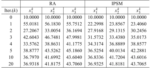
In Table 2, we show the first three components of each iterate for sake of comparison of IPSM with the relaxation algorithm RA given in [6].
RA IPSM
Iter.(k) x1k x2k x3k x1k x2k x3k
0 10.0000 10.0000 10.0000 10.0000 10.0000 10.0000 1 55.0181 56.1830 55.7512 22.2998 23.8567 23.4060 2 27.2067 33.0054 36.1694 27.9168 29.1315 30.2456 3 42.6043 46.7481 47.9981 31.5732 33.4380 35.0173 4 33.5762 38.8631 41.1775 34.3174 36.8889 38.8577 5 38.8777 43.5262 45.1860 36.5254 40.0134 42.2881 10 36.7970 41.6992 43.6040 36.8336 41.7204 43.6016 20 36.9318 41.8175 43.7060 36.9325 41.8181 43.7065
Table 2 – Example 4.2: Iterations of RA and IPSM, where
x∗=(36.912,41.842,43.705,42.665,39.182).
Again, despite the algorithms RA and IPSM obtain similar results at iteration 20, the computational effort is different.
Example 4.3. Consider two equilibrium problems given in [21], where
C =
(
x ∈R5 :
5 X
i=1
x1≥ −1, −5≤xi ≤5, i =1, . . . ,5
)
and the bifunction is of the form
f(x,y)= hP x+Qy+q,y−xi. (33)
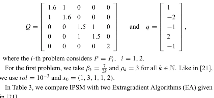
The matricesP,Qand the vectorqare defined by
P1=
3.1 2 0 0 0
2 3.6 0 0 0
0 0 3.5 2 0
0 0 2 3.3 0
0 0 0 0 2
, P2=
3.1 2 0 0 0
2 3.6 0 0 0
0 0 3.5 2 0
0 0 2 3.3 0
0 0 0 0 3
Q =
1.6 1 0 0 0
1 1.6 0 0 0
0 0 1.5 1 0
0 0 1 1.5 0
0 0 0 0 2
and q =
1 −2 −1 2 −1 ,
where thei-th problem considersP = Pi, i =1,2.
For the first problem, we takeβk = 27k andρk =3 for allk ∈N. Like in [21], we usetol=10−3andx0=(1,3,1,1,2).
In Table 3, we compare IPSM with two Extragradient Algorithms (EA) given in [21].
Scheme Iter.(k) Ls. step cpu(s)
EA-a 8 7 0.0562
EA-b 25 − 0.1148
IPSM 10 − 0.0006
Table 3 – Example 4.3: Problem 1.
In the second problem, we use P = P2,βk = 103k andρk = 3 for allk ∈ N. Like in [21], we taketol=10−3andx0=(1,3,1,1,2).
In Table 4, we compare IPSM with algorithm EA given in [21].
Scheme Iter.(k) Ls. step cpu(s)
EA-a 10 9 0.0605
IPSM 10 − 0.0006
Table 4 – Example 4.3: Problem 2.
Tables 3 and 4 show a good performance of algorithm IPSM.
Example 4.4. Consider the nonsmooth equilibrium problem defined by the bifunction f(x,y) = |y1| − |x1| + y22 − x22 and the constraint set C =
x ∈R2+ : x1+x2=1 . The optimal point is x∗ = (1 2,
1
2) and the partial
subdifferential of the equilibrium bifunction f is given by
∂2f(x,x)=
(1,2x2) if x1>0,
We use γk = max{1,kgkk} and kxk − x∗k ≤ 10−4 as stop criteria. In Table 5, we show our results by considering different initial points.
x10 x20 βk Iter.(k) cpu(s) 0.0000 1.0000 1/k 1 0.0057 0.1111 0.8889 9/k 8 0.0563 0.3333 0.6667 9/k 8 0.0560 0.6667 0.3333 4/k 5 0.0359 0.8889 0.1111 8/k 7 0.0478 1.0000 0.0000 1/k 1 0.0061
Table 5 – Example 4.4.
5 Concluding remarks
In this paper we have presented a subgradient-type method, denoted by IPSM, for solving equilibrium problems and established its convergence under mild assumptions.
Numerical results were reported for test problems given in the literature of computational methods for solving nonsmooth equilibrium problems. The com-parison with other two schemes has shown a satisfactory behavior of the algo-rithm IPSM in terms of the computational time.
Acknowledgements. We would like to thank two anonymous referees whose comments and suggestions greatly improved this work.
REFERENCES
[1] A. Auslender and M. Teboulle, Projected subgradient methods with non-Euclidean distances for non-differentiable convex minimization and variational
inequalities. Mathematical Programming,120(2009), 27–48.
[2] J.Y. Bello Cruz and A.N. Iusem, Convergence of direct methods for
paramono-tone variational inequalities. Computational Optimization and Applications,46
(2010), 247–263.
[4] E. Blum and W. Oettli,From optimization and variational inequalities to
equilib-rium problems. Math. Student,63(1994), 123–145.
[5] J.P. Crouzeix, P. Marcotte and D. Zhu, Conditions ensuring the applicability of
cutting-plane methods for solving variational inequalities. Mathematical
Pro-gramming,Ser. A 88(2000), 521–539.
[6] A. Heusinger and C. Kanzow, Relaxation Methods for Generalized Nash
Equi-librium Problems with Inexact Line Search. Journal of Optimization Theory and
Applications,143(2009), 159–183.
[7] H. Iiduka and I. Yamada,A Subgradient-type method for the equilibrium problem
over the fixed point set and its applications. Optimization,58(2009), 251–261.
[8] A.N. Iusem,On the Maximal Monotonicity of Diagonal Subdifferential Operators. Journal of Convex Analysis,18(2011), final page numbers not yet available. [9] A.N. Iusem and W. Sosa, New existence results for equilibrium problems.
Non-linear Analysis,52(2003), 621–635.
[10] A.N. Iusem and W. Sosa, Iterative algorithms for equilibrium problems. Opti-mization,52(2003), 301–316.
[11] A.N. Iusem and W. Sosa,On the proximal point method for equilibrium problems
in Hilbert spaces. Optimization,59(2010), 1259–1274.
[12] A.N. Iusem, G. Kassay and W. Sosa, On certain conditions for the existence
of solutions of equilibrium problems. Mathematical Programming,116 (2009),
621–635.
[13] I.V. Konnov, Application of the proximal point method to nonmonotone
equilib-rium problems. Journal of Optimization Theory and Applications, 119 (2003),
317–333.
[14] P.-E. Maingé, Strong Convergence of Projected Subgradient Methods for
Non-smooth and Nonstrictly Convex Minimization. Set-Valued Analysis, 16(2008),
899–912.
[15] L.D. Muu and T.D. Quoc, Regularization Algorithms for Solving Monotone Ky
Fan Inequalities with Application to a Nash-Cournot Equilibrium Model. Journal
of Optimization Theory and Applications,142(2009), 185–204.
[16] A. Nedi´c and A. Ozdaglar, Subgradient Methods for Saddle-Point Problems. Journal of Optimization Theory and Applications,142(2009), 205–228.
[18] T.T. Nguyen, J.J. Strodiot and V.H. Nguyen, The interior proximal
extragra-dient method for solving equilibrium problems. Journal of Global Optimization,
44(2009), 175–192.
[19] T.T. Nguyen, J.J. Strodiot and V.H. Nguyen, A bundle method for solving
equilib-rium problems. Mathematical Programming,116(2009), 529–552.
[20] S. Scheimberg and F.M. Jacinto, An extension of FKKM Lemma with an
appli-cation to generalized equilibrium problems. Pacific Journal of Optimization, 6
(2010), 243–253.
[21] D.Q. Tran, L.M. Dung and V.H. Nguyen, Extragradient algorithms extended to
![Table 1 gives the results obtained by IPSM algorithm and by the Relaxation Algorithm (RA) used in [6].](https://thumb-eu.123doks.com/thumbv2/123dok_br/18978200.456067/12.918.138.779.548.833/table-gives-results-obtained-ipsm-algorithm-relaxation-algorithm.webp)