ISSN 0101-8205 www.scielo.br/cam
Operational Tau approximation for a general class
of fractional integro-differential equations
S. KARIMI VANANI and A. AMINATAEI
Department of Mathematics, K.N. Toosi University of Technology, P.O. Box: 16315-1618, Tehran, Iran
E-mails: [email protected] / [email protected]
Abstract. In this work, an extension of the algebraic formulation of the operational Tau method (OTM) for the numerical solution of the linear and nonlinear fractional integro-differ-ential equations (FIDEs) is proposed. The main idea behind the OTM is to convert the fractional differential and integral parts of the desired FIDE to some operational matrices. Then the FIDE reduces to a set of algebraic equations. We demonstrate the Tau matrix representation for solving FIDEs based on arbitrary orthogonal polynomials. Some advantages of using the method, error estimation and computer algorithm are also presented. Illustrative linear and nonlinear experi-ments are included to show the validity and applicability of the presented method.
Mathematical subject classification: 65M70, 34A25, 26A33, 47Gxx.
Key words: spectral methods, operational Tau method, fractional integro-differential equa-tions, error estimation, computer algorithm of the method.
1 Introduction
The main object of this work is to solve the fractional integro-differential equa-tion of the following form:
Dαu(x) = F(x,u(x))+ Z x
0
G(x,t,u(t))dt,
m−1< α≤m, m∈N, x >0,
(1)
Bju(x) = λj, λj ∈R, j=0,1,2, . . . ,m−1, (2)
whereFandGare given smooth functions,Dαis a fractional differential operator of orderαin the Caputo’s sense,Bj; j=0,1, . . . ,m−1, aremsupplementary conditions andu(x)is a solution to be determined.
Differential and integral equations involving derivatives of non-integer order have shown to be adequate models for various phenomena arising in damping laws, diffusion processes, models of earthquake [1], fluid-dynamics traffic model [2], mathematical physics and engineering [3], fluid and continuum mechanics [4], chemistry, acoustics and psychology [5].
Some numerical methods for the solution of FIDEs are presented in the liter-ature. We can point out to the collocation method [6], Adomian decomposition method (ADM) [7]-[9], Spline collocation method [10], fractional differential transform method [11] and the method of combination of forward and central differences [12]. Out of the aforesaid methods, we desire to consider OTM for solving FIDEs.
Spectral methods provide a computational approach which achieved substan-tial popularity in the last three decades. Tau method is one of the most important spectral methods which is extensively applied for numerical solution of many problems. This method was invented by Lanczos [13] for solving ordinary dif-ferential equations (ODEs) and then the expansion of the method were done for many different problems such as partial differential equations (PDEs) [14]-[16], integral equations (IEs) [17], integro-differential equations (IDEs) [18] and etc. [19]-[22].
In this work, we are interested in solving FIDEs with an operational approach of the Tau method. Because in the Tau method, we are dealing with a system of equations wherein the matrix of unknown coefficients is sparse and can be easily invertible. Also, the differential and integral parts appearing in the equation is replaced by its operational Tau representation. Then, we obtain a system of algebraic equations wherein its solution is easy.
2 Basic definitions of the fractional calculus
In this section, we give some basic definitions and properties of the fractional calculus theory, which are used in this work [3, 23].
Definition 1. A real function u(x), x >0is said to be in the space Cμ,μ∈ R,
if there exists a real number p > μ, such that u(x) = xpv(x), wherev(x) ∈ C[0,∞)and it is said to be in the space Cμm iff u(m)(x)∈Cμ, m∈N.
Definition 2. The Riemann-Liouville fractional integral operator of order
α≥0, of a function u(x)∈Cμ,μ≥ −1, is defined as:
Jαu(x)= 1
Ŵ(α)
Z x
0
(x−t)α−1u(t)dt, α >0, x >0,
J0u(x)=u(x),
where Ŵ is the Gamma function. Some of the most important properties of operator Jαfor u(x)∈Cμ,μ≥ −1,α,β ≥0andγ >−1, are as follows:
i) JαJβu(x)= Jα+βu(x),
ii) JαJβu(x)= JβJαu(x),
iii) Jαxγ = Ŵ(γ +1) Ŵ(α+γ +1)x
α+γ.
Definition 3. The fractional derivative of u(x)in the Caputo’s sense is defined as:
Dαu(x)= Jm−αDmu(x)= 1
Ŵ(m−α)
Z x 0
(x −t)m−α−1u(m)(t)dt, (3)
when m−1< α≤m, m∈N, x >0, u(x)∈Cm
−1. 3 Operational Tau method
For any integrable functions ψ (x) andφ (x)on [a,b], we define the scalar producth, iby
hψ(x), φ (x)iw =
Z b
a
ψ (x)φ (x)ω(x)d x,
wherekψk2
w = hψ (x), ψ (x)iω andω(x)is a weight function. LetL2ω[a,b]be the space of all functions f : [a,b] →R, withkfk2ω <∞.
The main idea of the method is to seek a polynomial to approximateu(x) ∈ L2
ω[a,b]. Let φx = {φi(x)}∞i=0 = 8Xx be a set of arbitrary orthogonal poly-nomial bases defined by a lower triangular matrix8andXx =
1,x,x2, . . .T
.
Lemma 1. Suppose that u(x)is a polynomial as u(x) = P∞
i=0uixi = uXx,
then we have:
Dr(x)= d
r
d xru(x)=uM
rXx, r =0,1,2, . . . , (4)
xsu(x)=uNsXx, s =0,1,2, . . . , (5)
and Z x
a
u(t)dt =uPXx−uPXa, (6)
whereu = [u0,u1, . . . ,un, . . .], Xa =
1,a,a2, . . .T
, a ∈ RandM,Nand
Pare infinite matrices with only nonzero elements Mi+1,i =i+1,Ni,i+1 =1, Pi,i+1= i+11, i=0,1,2, . . . .
Proof. See [24].
Let us consider
u(x)=
∞
X
i=0
uiφi(x)=u8Xx, (7)
to be an orthogonal series expansion of the exact solution of equations (1) and (2), where u = {ui}∞i=0 is a vector of unknown coefficients, 8Xx is an orthogonal basis for polynomials inR.
Using equations (3), (4) and (7); we get:
Dαu(x)= Jm−αDm(u8Xx)= Jm−α(u8MmXx)=u8MmJm−α(Xx). (8) Using property iii) of Definition 2, we have:
Jm−α(Xx)=Jm−α(1),Jm−α(x), . . . ,Jm−α(xγ), . . . T
=
Ŵ(1)xm−α Ŵ(m−α+1),
Ŵ(2)xm−α+1 Ŵ(m−α+2), . . . ,
Ŵ(γ +1)xm−α+γ Ŵ(m−α+γ+1), . . .
T
=Ŵ5,
(9)
whereŴis an infinite diagonal matrix with elements
Ŵi,i =
Ŵ(i+1)
Ŵ(m−α+i+1),i =0,1, . . . ,
and
5=xm−α,xm−α+1, . . . ,xm−α+γ, . . .T. By approximatingxm−α+γ, γ =0,1, . . .;as follows:
xm−α+γ =
∞
X
i=0
aγ ,iφi(x)=aγ8Xx, aγ =
aγ ,0,aγ ,1,aγ ,2, . . .
,
we obtain:
5=a08Xx,a18Xx, . . . ,aγ8Xx, . . .T =A8Xx, A= [a0,a1, . . . ,aγ , . . .]T.
(10)
Substituting equation (10) in equation (9) and using equation (8); we obtain:
Dαu(x)=u8MmŴ5=u8MmŴA8Xx =uV8Xx, V=8MmŴA. (11) In next step, the aim is to linearize analytic functions F(x,u(x))and G(x,
t,u(t)). These functions can be written as:
F(x,u(x))=
∞
X
r=0
∞
X
p=0
fr pxrup(x), (12)
and
G(x,t,u(t))=
∞
X
r=0
∞
X
s=0
∞
X
p=0
Now, we state the following lemma and corollary.
Lemma 2. LetXx =
1,x,x2, . . .T
, u = [u0,u1,u2, . . .] be infinite vectors
and8=[φ0|φ1|φ2|. . .],φi are infinite columns of matrix8. Then, we have:
Xxu8Xx =UXx, (14)
whereUis an upper triangular matrix as:
Ui,j =
∞ X
k=0
ukφk,j−i, j≥i, i, j=0,1, . . . ,
0, j<i, i, j =0,1, . . . .
(15)
In addition, if we suppose that u(x)=u8Xx represents a polynomial, then for any positive integer p, the relation
up(x)=u8Up−1Xx, (16)
is valid.
Proof. We have:
Xxu8 = 1,x,x2, . . .Tuφ0|uφ1|uφ2|. . .
=
uφ0 uφ1 uφ2 ∙ ∙ ∙
uφ0x uφ1x uφ2x ∙ ∙ ∙
uφ0x2 uφ1x2 uφ2x2 ∙ ∙ ∙ .. . ... ... . .. , therefore
Xxu8Xx =
uφ0 uφ1 uφ2 ∙ ∙ ∙
uφ0x uφ1x uφ2x ∙ ∙ ∙ uφ0x2 uφ1x2 uφ2x2 ∙ ∙ ∙ .. . ... ... . ..
1,x,x2, . . .T
= P∞
i=0uφixi+0
P∞
i=0uφixi+1
P∞
i=0uφixi+2 .. . =
uφ0 uφ1 uφ2 ∙ ∙ ∙
0 uφ0 uφ1 ∙ ∙ ∙
0 0 uφ0 ∙ ∙ ∙
if we call the last upper triangular coefficient matrix asU, then we have:
Ui,j =
uφj−i, j ≥i, i, j =0,1, . . . , 0, j <i, i, j=0,1, . . . ,
= ∞ X
k=0
ukφk,j−i, j≥i, i, j=0,1, . . . ,
0, j<i, i, j =0,1, . . . .
Now, in order to prove equation (16), we apply induction. For p = 1, it is obvious thatu(x) = u8Xx. For p = 2, we rewriteu2(x) = u8Xxu8Xx = u8(Xxu8Xx)and using equation (14), we have:
u2(x)=u8UXx,
therefore, equation (16) is hold for p =2. Now, suppose that equation (16) is hold for p = k, then we must prove that the relation is valid for s = k +1. Thus,
uk+1(x)=uk(x)u(x)=(u8Uk−1Xx)(u8Xx)
=u8Uk−1(Xxu8Xx)=u8UkXx, So, equation (16) is proved.
We rewrite equation (12) as:
F(x,u(x))=
∞
X
r=0
∞
X
p=0
fr pxrup(x)=
∞
X
r=0
fr0xr +
∞
X
r=0
∞
X
p=1
fr pxrup(x),
The first summation can be considered as:
∞
X
r=0
fr0xr =fXx, f = [f00, f10, f20, . . .]. (17) For the second summation, using equations (5) and (16) yields:
∞
X
r=0
∞
X
p=1
fr pxrup(x)=
∞
X
r=0
∞
X
p=1
fr pxru8Up−1Xx =u8
∞
X
r=0
∞
X
p=1
fr pxrUp−1Xx
=u8
∞
X
r=0
∞
X
p=1
fr pUp−1NrXx =u8FXx, F=
∞
X
r=0
∞
X
p=1
fr pUp−1Nr
.
Therefore, we have:
F(x,u(x))=fXx +u8FXx = f8−1+u8F8−1
8Xx. (19)
In the same manner, we rewrite:
G(x,t,u(t)) =
∞
X
r=0
∞
X
s=0
∞
X
p=0
gr spxrtsup(t)
=
∞
X
r=0
∞
X
s=0
gr s0xrts+
∞
X
r=0
∞
X
s=0
∞
X
p=1
gr spxrtsup(t).
(20)
Using equation (5), the second summation is as:
∞
X
r=0
∞
X
s=0
∞
X
p=1
gr spxrtsup(t)=
∞
X
r=0
∞
X
s=0
∞
X
p=1
gr spxrtsu8Up−1Xt
=u8
∞
X
r=0
∞
X
s=0
∞
X
p=1
gr spxrtsUp−1Xt =u8
∞
X
r=0
∞
X
s=0
∞
X
p=1
gr spxrUp−1NsXt. (21)
Therefore,
Z x 0
G(x,t,u(t))dt =
∞
X
r=0
∞
X
s=0
gr s0xr
Z x 0
tsdt
+u8
∞
X
r=0
∞
X
s=0
∞
X
p=1
gr spxrUp−1Ns
Z x
0 Xtdt.
(22)
The first part easily can be written as follows:
∞
X
r=0
∞
X
s=0
gr s0xr
Z x
0
tsdt =
∞
X
r=0
∞
X
s=0
gr s0
xr+s+1
s+1 =gXx, (23)
where
gi =
0, i =0,
i−1
X
j=0 1
i− jgj(i−1−j)0, i ≥1.
Using equations (5) and (6), the second part of equation (22) is written as follows:
u8
∞
X
r=0
∞
X
s=0
∞
X
p=1
gr spxrUp−1NsPXx =u8
∞
X
r=0
∞
X
s=0
∞
X
p=1
gr spUp−1NsPMrXx (25)
=u8GXx, G=
∞
X
r=0
∞
X
s=0
∞
X
p=1
gr spUp−1NsPMr
. (26)
Thus, we have:
Z x
0
G(x,t,u(t))dt =(g+u8G)Xx = g8−1+u8G8−18Xx. (27) In addition, suppose that the supplementary conditions are generally as:
Bju(x)= l
X
i=0 q
X
k=0
bji ku(i)(xk)=λj, 0≤ xk ≤ x, j =0, . . . ,m−1.
Therefore, using equation (4) we have:
Bju(x)= l
X
i=0 q
X
k=0
bji ku8MiXxk =ubj =λj,
bj = l
X
i=0 q
X
k=0
bji k8MiXxk.
(28)
Using equations (11), (18) and (27) we replace equation (1) by the following operational form:
uV8Xx = f8−1+u8F8−1+g8−1+u8G8−1
8Xx. So, the residualR(x)of equation (1), can be written as:
R(x)=(f+g)8−1+u 8 (F+G)8−1−V8Xx =R8Xx, (29) where
Now, we set the residual matrixR=0 or we use the following inner products,
hR(x), φk(x)iw =0, k =0,1, . . . . (30)
Therefore an infinite system of algebraic equations is obtained. Since, some-where we require finite terms of approximation, then we must truncate the series to finite number of terms. Thus, we choosen+1−mof the first equations in Rand the following system is obtained:
Ri =0, i =0,1, . . . ,n−m, ubj =λj, j=0, . . . ,m−1, or
hR(x), φk(x)iw =0, k =0,1, . . . ,n−m, ubj =λj, j =0, . . . ,m−1.
Solving the aforesaid system yields the unknown vectoru = [u0,u1, . . . ,un]. This is the so-called operational Tau method which is applicable for finite, infinite, regular and irregular domains.
We summarize OTM in the following algorithm.
Algorithm of the method:
Step 1: Choose suitable orthogonal basesφ (x) = {φi(x)}ni=0 and find non-singular coefficient matrix8and the compute8−1.
Step 2:Consideru(x)=u8Xx as the series expansion of exact solution. Step 3:Use equations (4) through (11) to evaluate matrixV.
Step 4:Use equations (18) and (27) to obtain vectors f,gand matricesF,G. Step 5:Compute matrixRfrom residual term R(x,t)and setR=0. Step 6:Imposemsupplementary conditionsubj =λjand solve the obtained system.
4 Some orthogonal polynomials
4.1 Legendre polynomials
The well-known Legendre polynomials are defined as follows:
P0(x)=1,P1(x)=x, x ∈ [−1,1],
Pi(x)=
2− 1 i
x Pi−1(x)−
1−1 i
Pi−2(x), i≥2.
They are orthogonal on the interval[−1,1]with respect to the weight function w(x)=1 and satisfy:
Z 1
−1
w(x)Pm(x)Pn(x)d x =
2
2n+1, m =n,
0, m 6=n.
Since the interval of orthogonality of these polynomials may differ with the domain of the problem, we must shift the polynomial to the desired interval. Thus, to construct the shifted Legendre polynomials on arbitrary interval[0,h], it is sufficient to do the change of variable: x → 2xh−h. So, the shifted Legendre polynomials are defined as follows:
P0(x)=1,P1(x)=
2x −h
h , x ∈ [0,h],
Pi(x)=
2−1 i
2x −h h
Pi−1(x)−
1−1 i
Pi−2(x), i ≥2,
and satisfy:
Z h
0
w(x)Pm(x)Pn(x)d x =
h
2n+1, m=n,
0, m6=n.
4.2 Laguerre polynomials
Laguerre polynomials are defined as follows:
L0(x)=1, L1(x)=1−x, x ∈ [0,∞),
Li(x)=
2i−1−x i
Li−1(x)−
i−1
i
They are orthogonal on the interval[0,∞)with respect to the weight function w(x)=e−x and satisfy:
Z ∞
0
w(x)Lm(x)Ln(x)d x =
1, m=n,
0, m6=n.
5 Error estimation
In this section, an error estimation for the approximate solution of equation (1) with supplementary conditions (2) is obtained. Let us callen(x)=u(x)−un(x) as the error function of the approximate solutionun(x)tou(x)whereu(x)is the exact solution of equation (1). Hence,un(x)satisfies the following equations:
Dαun(x) = F(x,un(x))+
Z x
0
G(x,t,un(t))dt+Hn(x),
m−1< α≤m,
(31)
Bjun(x)=λj, λj ∈R, j=0,1,2, . . . ,m−1. (32)
The perturbation term Hn(x) can be obtained by substituting the computed solutionun(x)into the equation:
Hn(x)=Dαun(x)−F(x,un(x))−
Z x
0
G(x,t,un(t))dt.
We proceed to find an approximationen,N(x)to the error functionen(x)in the same way as we did before for the solution of equation (1). Note that N is the degree of approximation ofun(x). By subtracting equations (31) and (32) from equations (1) and (2), respectively we have:
Dα(u(x)−un(x))=F(x,u(x)−un(x))
+ Z x
0
G(x,t,u(t)−un(t))dt−Hn(x),
Bj(u(x)−un(x))=0,
or
Dα(en(x))=F(x,en(x))+ Z x
0
G(x,t,en(t))dt−Hn(x),
It should be noted that in order to construct the approximateen,N(x)toen(x), only the related equations like as equations (7) through (31) needs to be recomputed and the structure of the method remains the same.
6 Illustrative numerical experiments with some comments
In this section, four experiments of linear and nonlinear FIDEs are given to illus-trate the results. In all experiments, we consider the shifted Legendre polyno-mials as basis functions for finite domains and Laguerre polynopolyno-mials for infinite domains. The computations associated with the experiments discussed above were performed in Maple 13 on a PC with a CPU of 2.4 GHz.
Experiment 6.1. Consider the following FIDE [6, 7]:
D0.75u(x)= −
x2ex 5
u(x)+ x
2.25 Ŵ(3.25) +
Z x
0
texu(t)dt, x >0, (33)
with the initial condition:u(0)=0 The exact solution is: u(x)=x3.
We have solved this experiment using OTM with Laguerre polynomials and some approximations are obtained as follows:
n=0: u= [0], u0(x)=0,
n=1: u= [−1.536502,1.536502], u1(x)= −1.536502x,
n=2: u= [−0.701605,1.413861,−0.712256], u2(x)=0.010651x−0.356128x2, n=3: u= [6,−18,18,−6], u4(x)=x3,
n=4: u= [6,−18,18,−6,0], u4(x)=x3, n=5: u= [6,−18,18,−6,0,0], u5(x)=x3,
. .
. ... ...
and so on.
Thus, we haveu(x)=x3which is the exact solution of the problem. Experiment 6.2. Consider the following nonlinear FIDE [8]:
Dαu(x)=1+ Z x
0
with the boundary conditions:
u(0)=u′(0)=1,
u(1)=u′(1)=e.
The only case which we know the exact solution forα =4 is: u(x)=ex. We have solved this experiment forn=7 with differentαand have compared it with the closed form series solutions of the exact solution obtained by ADM [8]. The comparison is shown in Table 1.
α=3.25 α=3.5 α=3.75
x uADM uOTM uADM uOTM uADM uOTM
0.0 1.000000 1.000000 1.000000 1.000000 1.000000 1.000000 0.1 1.106551 1.107575 1.106750 1.106693 1.106151 1.105930 0.2 1.223931 1.225838 1.224323 1.224220 1.223227 1.222813 0.3 1.353200 1.355724 1.353755 1.353600 1.352308 1.351741 0.4 1.495600 1.498421 1.496270 1.496050 1.494635 1.493962 0.5 1.652553 1.655348 1.653273 1.652982 1.651615 1.650890 0.6 1.825654 1.828146 1.826354 1.826006 1.824823 1.824110 0.7 2.016687 2.018671 2.017294 2.016931 2.016023 2.015390 0.8 2.227634 2.228987 2.228084 2.227770 2.227176 2.226696 0.9 2.460690 2.461367 2.460931 2.460744 2.460458 2.460196 1.0 2.718281 2.718281 2.718281 2.718281 2.718281 2.718281
Table 1 – Comparison of the solutions of ADM and OTM for differentαof Experiment 6.2.
From the numerical results in Table 1, it is easy to conclude that obtained results by OTM are in good agreement with those obtained using the ADM. In this experiment, the exact solution is not known, so a main question arises that which method is more accurate. We conclude that OTM is more accurate by considering the following notation and discussion.
Note 1. In the theory of fractional calculus, it is obvious that when the frac-tional derivativeα (m−1 < α ≤ m)tends to positive integer numberm, then the approximate solutioncontinuouslytends to the exact solution of the problem with derivationm.
so the values forα = 3.5 must be less than the values forα = 3.75. But this fact have not occurred for ADM solutions but for OTM solutions, we have the reduction in the results. Therefore OTM is more reliable than ADM.
Moreover, forα =4, using Legendre polynomials, the following sequences of approximate solution is obtained:
n=4: u= 103 60 , 101 120, 23 168, 1 80, 1 1680 ,
u4(x)=1+x+
x2 2 + x3 6 + x4 24,
n=5: u= 1237 720 , 473 560, 281 2016, 59 4320, 1 1120, 1 30240 ,
u5(x)=1+x+
x2 2 + x3 6 + x4 24 + x5 120,
n=6: u= 433 252, 1893 2240, 1691 12096, 1 72, 3 3080, 1 20160, 1 665280 ,
u6(x)=1+x+
x2 2 + x3 6 + x4 24 + x5 120+ x6 720, .. . ...
and so on.
Thus, we obtain:
un(x)=1+x+
x2
2! + x3
3! + x4
4! + ∙ ∙ ∙ + xn n!.
This has the closed formu(x)=ex, which is the exact solution of the problem. Thus, for positive integer derivatives, if the exact solution exists, then OTM produces its series solution.
Experiment 6.3. Consider the following nonlinear FIDE:
Dαu(x) = x3 −1+esinx
−sinx− Z x
0
x3cost eu(t)dt,
x >0, 1< α≤2,
with the initial conditions:
u(0)=0,u′(0)=1.
The only case which we know the exact solution forα =2 isu(x)=sinx. We have solved this experiment for n = 5 with different α and have used Laguerre polynomials as basis functions. The results are given in Table 2.
x α=1.25 α=1.5 α=1.75 α=2 uExact
0.0 0.000000 0.000000 0.000000 0.000000 0.000000 0.1 0.097355 0.098677 0.099419 0.099833 0.099833 0.2 0.188547 0.193716 0.196812 0.198669 0.198669 0.3 0.272375 0.283807 0.290975 0.295520 0.295520 0.4 0.347526 0.367799 0.380815 0.389418 0.389418 0.5 0.412246 0.444601 0.465333 0.479427 0.479425 0.6 0.464013 0.513081 0.543605 0.564648 0.564642 0.7 0.499207 0.571968 0.614770 0.644233 0.644217 0.8 0.512786 0.619749 0.678009 0.717397 0.717356 0.9 0.497956 0.654568 0.732528 0.783420 0.783326 1.0 0.445845 0.674130 0.777544 0.841666 0.841470
Table 2 – OTM solutions forn=5 with differentαof Experiment 6.3.
Forα = 2, using Laguerre polynomials, the following sequence of approxi-mate solution is obtained:
n=0: u=[0], u0(x)=0,
n=1: u=[1,−1], u1(x)=x,
n=2: u=[1,−1,0], u2(x)=x,
n=3: u=[0,2,−3,1], u3(x)=x− x
3 6 ,
n=4: u=[0,2,−3,1,0], u4(x)=x−
x3 6 ,
n=5: u=[1,−3,7,−9,5,−1], u5(x)=x−
x3
6 +
x5
120,
n=6: u=[1,−3,7,−9,5,−1,0], u6(x)=x−
x3
6 +
x5 120, ..
. ... ...
Thus, we obtain:
u2n+1(x)=x−
x3
3! + x5
5! + ∙ ∙ ∙ +(−1)
n x 2n+1 (2n+1)!.
This has the closed formu(x)=sinx, which is the exact solution of the problem.
Experiment 6.4. Consider the following nonlinear FIDE:
Dαu(x) = e−x +2
3
e−32x−1
+
Z x
0
e−tpu(t)dt,
0≤ x ≤1, 1< α≤2,
(36)
with the initial conditions:
u(0)=1,u′(0)= −1.
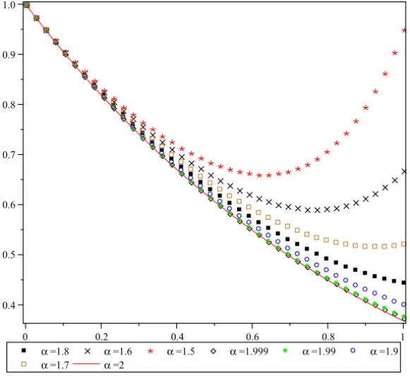
The only case which we know the exact solution forα =2 is: u(x)=e−x. We have solved this experiment forn = 4 with differentα and used shifted Legendre polynomials as basis functions. Figure 1 shows the approximate solu-tions and illustrates the aforesaid fact given by note 1.
The following figure illustrates the convergency of the method and the fact that the method tends continuously to the exact solution if fractional derivations tend to an integer order.
For α = 2, using shifted Legendre polynomials, the following sequence of approximate solution is obtained:
n =0: u= [1], u0(x)=1,
n =1: u= 1
2,− 1 2
, u1(x)=1−x,
n =2: u=
2 3,−
1 12,
1 2
, u2(x)=1−x+
x2
2 ,
n =3: u=
5 8,−
13 40,
1 24,−
1 120
, u3(x)=1−x+ x
2
2 −
x3
6 , ..
. ... ...
Figure 1 – The graphs of the approximate solutions forn = 4 with different α of
Experiment 6.4.
Thus, we obtain:
un(x)=1−x+
x2 2! −
x3
3! + ∙ ∙ ∙ +(−1)
nx n
n!.
This has the closed form u(x) = e−x, which is the exact solution of the problem.
7 Conclusion
The most important ones are the simplicity of the method, reducing the com-putations using orthogonal polynomials and having low run time of its algo-rithm. Furthermore, this method yields the desired accuracy only in a few terms in a series form of the exact solution. All of these advantages of the OTM to solve nonlinear problems assert the method as a convenient, reliable and powerful tool.
REFERENCES
[1] J.H. He, Nonlinear oscillation with fractional derivative and its applications. In: International Conference on Vibrating Engineering, Dalian, China (1998), 288–291.
[2] J.H. He, Some applications of nonlinear fractional differential equations and their approximations.Bull. Sci. Technol.,15(1999), 86–90.
[3] I. Podlubny,Fractional Differential Equations.Academic Press, New York (1999).
[4] F. Mainardi, Fractals and Fractional Calculus Continuum Mechanics.Springer Verlag, (1997), 291–348.
[5] W.M. Ahmad and R. El-Khazali, Fractional-order dynamical models of love.
Chaos, Solitons & Fractals,33(2007), 1367–1375.
[6] E.A. Rawashdeh, Numerical solution of fractional integro-differential equations by collocation method.Applied Mathematics and Computation,176(2005), 1–6.
[7] R.C. Mittal and R. Nigam, Solution of fractional integro-differential equations by adomian decomposition method.Int. J. of Appl. Math. and Mech., 4(2008), 87–94.
[8] S. Momani and M.A. Noor, Numerical methods for fourth-order fractional integro-differential equations. Applied Mathematics and Computation, 182 (2006), 754–760.
[9] W.G. El-Sayed and A.M.A. El-Sayed, On the functional integral equations of mixed type and integro-differential equations of fractional orders. Applied Mathematics and Computation,154(2004), 461–467.
[10] A. Pedas and E. Tamme,Spline collocation method for integro-differential equa-tions with weakly singular kernels.Journal of Computational and Applied Math-ematics,197(2006), 253–269.
[12] M.F. Al-Jamal and E.A. Rawashde,The Approximate Solution of Fractional Inte-gro-Differential Equations.Int. J. Contemp. Math. Sciences,4(2009), 1067–1078.
[13] C. Lanczos, Trigonometric interpolation of empirical and analytical functions.
J. Math. Phys.,17(1938), 123–199.
[14] K.M. Liu and E.L. Ortiz, Numerical solution of eigenvalue problems for partial differential equations with the Tau-lines method.Comp. Math. Appl. B,12(1986), 1153–1168.
[15] E.L. Ortiz and K.S. Pun, Numerical solution of nonlinear partial differential equations with Tau method.J. Comp. Appl. Math.,12(1985), 511–516.
[16] E.L. Ortiz and H. Samara, Numerical solution of partial differential equations with variable coefficients with an operational approach to the Tau method.Comp. Math. Appl.,10(1984), 5–13.
[17] M.K. EL-Daou and H.G. Khajah, Iterated solutions of linear operator equations with the Tau method.Math. Comput.,66(217) (1997), 207–213.
[18] J. Pour-Mahmoud, M.Y. Rahimi-Ardabili and S. Shahmorad, Numerical solution of the system of Fredholm integro-differential equations by the Tau method.Applied Mathematics and Computation,168(2005), 465–478.
[19] K.M. Liu and E.L. Ortiz, Approximation of eigenvalues defined by ordinary dif-ferential equations with the Tau method.Matrix Pencils, Springer, Berlin, (1983), 90–102.
[20] K.M. Liu and E.L. Ortiz, Tau method approximation of differential eigenvalue problems where the spectral parameter enters nonlinearly. J. Comput. Phys., 72(1987), 299–310.
[21] K.M. Liu and E.L. Ortiz, Numerical solution of ordinary and partial functional-differential eigenvalue problems with the Tau method. Computing, 41 (1989), 205–217.
[22] E.L. Ortiz and H. Samara, Numerical solution of differential eigenvalue problems with an operational approach to the Tau method.Computing,31(1983), 95–103.
[23] S. Samko, A. Kilbas and O. Marichev, Fractional Integrals and Derivatives.
Gordon and Breach, Yverdon (1993).