A Mathematical Model for the Removal of Organic Mater in
Stabilization Ponds
Waldir Medri
*and Vandir Medri
Universidade Estadual de Londrina, Departamento de Matemática Aplicada, Campus Universitário, CEP 86510-990, Londrina – PR, Brazil
ABSTRACT
This work presents an application to systemize the construction of ponds systems for treatment of domestic sewage. It consisted of two anaerobic ponds operated in parallel during May/97 to April/99. These were connected in series with a chicaned facultative pond. The treatment system was controlled with samples collected from the crude sewage (compound sample), in the affluents and effluents of the ponds and along the flux of the anaerobic and facultative ponds. The following parameters were analyzed: pH, Biochemical Oxygen Demand, Chemical Oxygen Demand, Total Solids, Sedimentable Solids, Total Coliforms, Ox ygen Consumed in Acid Medium (OCAM) and temperature.
Key words: Stabilization ponds, mathematical model, optimization
* Author for correspondence
INTRODUCTION
The stabilization ponds are modeled to keep wastewater until the wished effluent is obtained by the activity of microorganisms present in the system. The treatment process is realized by the capacity of microorganisms to break complex organic molecules into more simple inorganic substances during the cellular synthesis processes (Dorego & Leduc, 1996).
Stabilization ponds systems are quite old techniques for waste treatment. These systems have some advantages over the conventional treatments such as: low capital, operational and maintenance costs and simplified operation. The disadvantage is that it needs a big area. This article presents models of capital costs (costs with land area occupied by the ponds system and its construction) and maintenance costs, in order to optimize the system, objecting to minimize of the
total cost with adequate final effluent in terms of organic mater.
METHODS AND MATERIALS
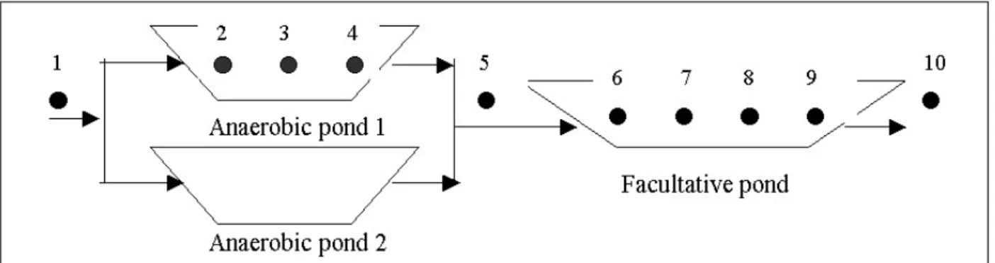
Figure 1 - Wastewater treatment system of Ibiporã/Pr South Zone
Table 1 - Physical and operational characteristics of the ponds
DIMENSIONS P O N D S Anaerobic pond 1 Anaerobic pond 2 Facultative pond
Surface length (m) 154 154 210
Bottom length (m) 149 147 209
Surface width (m) 22 22 51
Bottom width (m) 19 19 48
Average surface (m2) 3,106 3,085 10,370
Depth (m) 2 1.9 1.5
Volume (m3) 6,211 5,862 15,555
Discharge (m3/d) 743 743 1486
Detention time (d) 8.3 7.9 10.5
Control and Physico – Chemical Analysis
The crude sewage control was realized every hour from the 10th to 17th of June/1996 in an amount of 168 collections as the samples were compound type (point 1), while for the anaerobic ponds effluents AP1 and AP2 (point 5) and the facultative pond FP (point 10), the samples were collected every 15 days between May/1997 and April/1999. For the samples collected from ponds AP1 (2, 3, 4) and FP (6, 7, 8, 9) the control was realized between May/1998 and April/1999. Figure 1 presents the points of sample collection. Following parameters were analyzed: pH, Biochemical Oxygen Demand (BOD), Chemical Oxygen Demand (COD), Total Solids (TS), Sedimentable Solids (SS), Total Coliforms (TC-24h), Total Coliforms (TC-48h), Oxygen Consumed in Acid Medium (OCAM) and temperature, according to Standard Methods for Examination of Water and Wastewater, 1992).RESULTS AND DISCUSSIONS
The average, minimum and maximum values obtained from the domestic sewage treatment
system of SAMAE between May/1997 and April/1999 are presented in Table 2.
Operational Datas
It was observed that the average results obtained along the flux of the anaerobic pond characterized a system closer to the Complete Mixture than to
the Piston Flux, because it had not a high
affluents and effluents of the ponds Average, Minimum
and Maximum of
AP1 - AP2 FP
BOD5
(mg/l)
661.8 - 98.8 661.8 - 32.0 661.8 - 180.0
98.8 - 61.4 32.0 - 20.0 180.0 - 124.0 COD
(mg/l)
1,289.4 - 231.9 1,289.4 - 47.0 1,289.4 - 538.0
231.9 - 149.2 47.0 - 37.0 538.0 - 393.0 TS
(mg/l)
1,088.6 - 335.9 1,088.6 - 120.0 1,088.6 - 730.0
335.9 - 267.2 120.0 - 80.0 730.0 - 720.0 SS
(mg/l)
10.6 - 0.3 10.6 - 0.01
10.6 - 1.3
0.3 - 0.1 0.01 - 0.01 1.3 - 0.5 OD
(mg/l)
-
A B C 0.1 1.0 1.9
0 0 0 2.4 7.6 10.4 OCAM
(mg/l)
103.6 - 44.6 103.6 - 23.0 103.6 - 80.0
44.6 - 34.1 23.0 - 11.0 80.0 - 83.0
pH 6.98 - 7.2
6.98 - 7.0 6.98 - 7.6
7.2 - 7.7 7.0 - 7.3 7.6 - 8.2 TC – 24 hours
(nmp/100 ml)
1.75E8 - 6.14E6 1.75E8 - 0.03E6 1.75E8 - 35.00E6
6.14E6 - 4.26E6 0.03E6 - 0.04E6 35.00E6 - 92.00E6 TC – 48 hours
(nmp/100 ml)
2.85E8 - 16.77E6 2.85E8 - 0.33E6 2.85E8 - 92.00E6
16.77E6 - 5.58E6 0.33E6 - 0.09E6 92.00E6 - 92.00E6 Temperature
(0 C)
22.1 16.5 27.0
22.4 17.0 28.0
The anaerobic ponds affluents were assemblage samples, and the effluents were a common point (facultative pond affluent).Average environmental temperature during the control period was 20.4 oC, with minimum of 13.5oC and maximum of 26.5oC.
Pond Efficiency
i i
i i i
t
k
t
k
E
.
1
.
+
=
(1)where: Ei was the removal efficiency of pond i, and ti
were the detention time, in days.
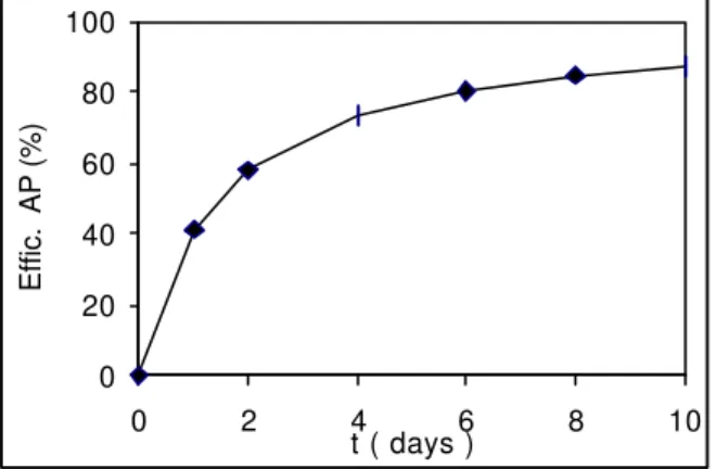
Although the BOD removal kinetic was the same for the anaerobic and facultative ponds (first order kinetic), the higher was the medium concentration the higher was the BOD removal rate. The adjusted efficiency curves of the anaerobic ponds (AP) and the facultative one (FP) are presented in Figures 2 and 3.
0 20 40 60 80 100
0 2 4 6 8 10
t ( days )
Effic. AP (%)
Figure 2 - Relation between the BOD efficiency and detention time in the pond AP
0 10 20 30 40 50
0 2 4 6 8 10 12
t ( days )
Effic. FP (%)
Figure 3 - Relation between the BOD efficiency and detention time in the pond FP
Detention Time
The detention time of each stabilization pond is expressed by:
Q
V
t
ii
=
(2) where: Vi is the volume the pond i, in m3, and Q is thesystem capacity, in m3/day.
Costs Models
In the economical analysis of the wastewater treatment system, the total cost includes costs with the land occupied by the system, construction and maintenance. Therefore it is necessary to obtain the costs models, so that:
CT = Cl + Cc + Cm (3)
where: CT is the total cost of the system; Cl is the land
cost; Cc is the construction cost and Cm is the
maintenance cost.
The initial investment includes the following costs: a) acquisition of the land occupied by the system plus 50% for the traffic of vehicles and/or people; b) ponds construction including the land cleanse, mechanical excavation, transport of the exceeding land and compaction.
Land Cost
The land cost is associated not only to the area occupied by the ponds system, but also to its adjacent area. Thus, the mathematical model that better represents this cost is expressed by the equation:
Cli = 1.5 γi Pl Vi (4)
where: Cli is the cost of the land occupied by pond i and
its adjacent area, in US$; Pl is the land price, in US$/m2; γi is the relation between the surface and the
volume of pond i, in m2/m3.
Construction Cost
The adjusted mathematical model that better describes the cost of the earth transport is given by (Medri, 1997):
Cci= 5.914 Vi0.95 (5)
where: Cci is the construction cost of pond i, in US$.
Maintenance Cost
83 . 0 1
)
(
164
.
0
n ii i
m
V
C
∑
=
=
φ
γ
(6)where, n n
r
r
r
)
1
(
1
)
1
(
+
−
+
=
Φ
(7)and Cm is the total cost of the ponds system
maintenance, in US$; φ is the factor of the present value; r is the annual interest rate and n is the life time of the ponds, in years.
From equation (4) to (6), it is possible to calculate the ponds cost:
Ci = 1.5 γi Pl Vi +5.914 Vi0.95 + Cmi (8)
From equation (1) to (2), it is possible to have the ponds volume:
Vi = Q Ei [ki (1- Ei)]-1 (9)
Substituting equation (9) in equation (8), it gives the cost ponds:
Ci = 1.5 γi Pl Q Ei [ki (1- Ei)]-1 +
5.914{Q Ei [ki (1- Ei)]-1}0.95 + Cmi (10)
where Ci is the cost the pond i, in US$.
land, construction, maintenance, and the system restriction condition is the wished final quality of the effluent, so that:
∑
==
n i i TC
C
Min
1 (11)1
0
:
.
.
≤
≤
≥
i w OE
E
E
to
s
where: CT is the system total cost, in US$; Eo is the obtained efficiency and Ew is the wished efficiency.
Thus, considering two anaerobic ponds in parallel followed by a facultative one, as the studied system, the problem can be formulated as followed: 83 . 0 1 3 3 3 3 1 2 2 2 2 1 1 1 1 1 95 . 0 1 3 3 3 1 3 3 3 3 95 . 0 1 2 2 2 1 2 2 2 2 95 . 0 1 1 1 1 1 1 1 1 1
]}
))
1
(
(
)
))
1
(
(
))
1
(
(
(
5
.
0
[
5
.
0
{
164
.
0
.
}
)]
1
(
[
{
914
.
5
)]
1
(
[
5
.
1
}
)]
1
(
[
5
.
0
{
914
.
5
)]
1
(
[
5
.
1
5
.
0
}
)]
1
(
[
5
.
0
{
914
.
5
)]
1
(
[
5
.
1
5
.
0
− − − − − − − − −−
+
−
+
−
+
−
+
−
+
−
+
−
+
−
+
−
=
E
k
E
Q
E
k
E
E
k
E
Q
E
k
E
Q
E
k
E
Q
Pl
E
k
E
Q
E
k
E
Q
Pl
x
E
k
E
Q
E
k
E
Q
Pl
x
MinC
Tγ
γ
γ
φ
γ
γ
γ
wE
E
E
E
to
s
.
.
:
1
−
[
1
−
0
.
5
(
1+
2)](
1
−
3)
≥
1
0
;
1
0
;
1
Practical Application
Making a study for 15 years and admitting interest rate of 10% per year, the factor of the present φ value given by equation (7) would be alike 95. Considering the average concentrations in the entrace and exit of the anaerobic (AP1) and facultative (FP) ponds and their detention time, the degradation constants k(BOD) were: 0.703 d-1 for ponds AP1 and 0.058 d-1 for the FP. These values
were determined with average temperature around 22oC.
Land price in north Paraná region is approximately R$ 2,500.00/ha. Considering two years (1998-1999), the devaluation of Real comparing to American dollar approximately 70%, and relation between surface area and volume of each pond as γ1=0.55; γ2 = 0.58 e γ3 = 0.69 m2/m3,for ponds AP1, AP2 and FP respectively, and admitting only the reduction of the organic matter (BOD), the mathematical model of model minimization is:
}
)]
))
1
(
058
.
0
(
69
.
0
)
))
1
(
703
.
0
(
58
.
0
))
1
(
703
.
0
(
55
.
0
(
5
.
0
(
5
.
0
[
164
.
0
95
7
.
0
]
))
1
(
058
.
0
(
[
914
.
5
7
.
0
)]
1
(
058
.
0
[
250
.
0
69
.
0
5
.
1
]
))
1
(
703
.
0
(
5
.
0
[
914
.
5
7
.
0
)]
1
(
703
.
0
[
250
.
0
58
.
0
5
.
1
5
.
0
]
))
1
(
703
.
0
(
5
.
0
[
914
.
5
7
.
0
)]
1
(
703
.
0
[
250
.
0
55
.
0
5
.
1
5
.
0
83 . 0 1 3 3 1 2 2 1 1 1 95 . 0 1 3 3 1 3 3 95 . 0 1 2 2 1 2 2 95 . 0 1 1 1 1 1 1 − − − − − − − − −−
+
−
+
−
+
−
+
−
+
−
+
−
+
−
+
−
=
X
X
Q
X
X
X
X
Q
x
x
X
X
Q
x
X
X
Q
x
x
X
X
Q
x
X
X
Q
x
x
x
X
X
Q
x
X
X
Q
x
x
x
MinC
T85
.
0
)
1
)](
(
5
.
0
1
[
1
:
.
.
to
−
−
X
1+
X
2−
X
3≥
s
1
,
,
0
≤
X
1X
2X
3≤
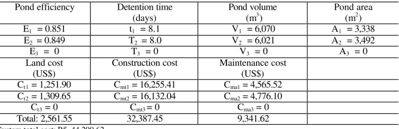
Table 3 - presents the physical characteristics of ponds and costs with land, construction and system maintenance, supposing discharge of 1,500 m3/day and system efficiency of 85%.
Pond efficiency Detention time
(days) Pond volume (m3) Pond area (m2)
E1 = 0.851 t1 = 8.1 V1 = 6,070 A1 = 3,338
E2 = 0.849 T2 = 8.0 V2 = 6,021 A2 = 3,492
E3 = 0 T3 = 0 V3 = 0 A3 = 0
Land cost
(US$) Construction cost (US$) Maintenance cost (US$) Ct1 = 1,251.90 Cmt1 = 16,255.41 Cma1 = 4,565.52 Ct2 = 1,309.65 Cmt2 = 16,132.04 Cma2 = 4,776.10
Ct3 = 0 Cmt3 = 0 Cma3 = 0
Total: 2,561.55 32,387.45 9,341.62
System total cost: R$ 44,290.62
As expected, the model excluded the secondary facultative pond, because it presented a low performance in the removal of the organic matter (BOD).
CONCLUSIONS
The results obtained from the stabilization system, consisting of two anaerobic ponds and a chicaned
facultative pond, treating the domestic sewage enabled to conclude that:
- the removal efficiency of the carbonaceous pollution (BOD and COD) was realized specially in the anaerobic ponds, with removal of 85% of BOD and 82% of COD with detention time of 8.1 days, while the facultative pond had 10.5 days of detention time and removed only 38% of BOD and 36% of COD;
treatment of domestic sewage, the degradation constant value of BOD of the anaerobic pond was highest than the facultative pond, because it was biodegraded easily, and the remained organic matter was more resistant to biodegradation. The total cost (cost with land, construction and maintenance) of the ponds system: two anaerobic ponds in parallel (AP1 and AP2), followed by a facultative (FP) in series was US$ 42,290.62 for an efficiency of 85% of BOD, discharge of 1,500 m3/day, and admitting interest rate off 10% per year during 15 years.
RESUMO
Este trabalho apresenta uma aplicação para sistematizar a construção de sistemas de lagoas para tratamento de esgoto doméstico. O sistema consiste de duas lagoas anaeróbias operando em paralelo durante o período de maio/97 até abril/99. Estas lagoas eram conectadas em série com uma lagoa facultativa chicaneada. O sistema de tratamento foi monitorado com amostra coletadas no esgoto bruto (amostra composta), nos afluentes e efluentes das lagoas e ao longo dos fluxos das lagoas anaeróbia e facultativa. Os seguintes parâmetros foram analisados: pH, Demanda Bioquímica de Oxigênio (DBO), Demanda
hidraulic flow patterns in facultative aerated lagoons. Wat. Sci. Tech., 34(11), 99-106.
Hess, M. L. (1980), Aspectos praticos de deseño de lagunas de estabilizacion. In. Proyecto de desarrolo tecnologico de las instituciones de abastecimiento de agua potable y alcantarillado, Lima, Peru. CEPIS, 15-26.
Kezhao, Z. (1994), pond system optimization. In: International Conference, Anais... Singapure Rai, 275-286.
Medri, W. (1997), Modelagem e otimização de sistemas de lagoas de estabilização para tratamento de dejetos suíno. Dr. Thesis, Universidade Federal de Santa Catarina, Florianópolis/SC Brasil.
Meisheng, N.; Kezhao, Z. and Lianquan, L. (1992), System optimization of stabilization ponds. Wat. Sci. Tech., 26(7- 8), 1679-1688.
Standard Methods (1992), for the Examination of Water and Wastewater. 18th. Washington, 1268 p.
Von Sperling, M. (1996), Princípios do tratamento
biológico de águas agoas de
estabilização DESA-UFMG. 134 p.
Yang, P. Y.; Khan, E.; Gan, G.; Paquin, L and Liang, T. (1997), A prototippe small swine waste treatment system for land limited and tropical application. Wat. Sci. Tech., 35(6), 145-152.