M
ESTRADO
E
CONOMIA
M
ONETÁRIA E
F
INANCEIRA
T
RABALHO
F
INAL DE
M
ESTRADO
D
ISSERTAÇÃO
S
HOULD
C
ENTRAL
B
ANKS
I
NCREASE THE
I
NFLATION
T
ARGET
?
M
ÁRIO
A
NDRÉ
S
ANTOS DE
O
LIVEIRA
M
ESTRADO EM
E
CONOMIA
M
ONETÁRIA E
F
INANCEIRA
T
RABALHO
F
INAL DE
M
ESTRADO
D
ISSERTAÇÃO
S
HOULD
C
ENTRAL BANKS
I
NCREASE THE
I
NFLATION
T
ARGET
?
M
ÁRIO
A
NDRÉ
S
ANTOS DE
O
LIVEIRA
O
RIENTAÇÃO
:
B
ERNARDINO
A
DÃO
(B
ANCO DE
P
ORTUGAL
)
Lisbon School of Economics and Management - University of Lisbon
Master’s in Monetary and Financial Economics
Dissertation
Should Central Banks Increase the Inflation Target?
M´ario Andr´e Santos de Oliveira†
Supervisor: Bernardino Ad˜ao (Bank of Portugal)
Abstract
Typically when central banks face economic slowdowns they use the
inter-est rate channel to boost economies. However, we have seen that if the nominal
interest rate is already at low levels, then their capacity to invert such
eco-nomic slowdowns is little. The main objective of this dissertation is to study
whether increasing the inflation target can increase the capacity of central
banks to invert economic downturns. Specifically, we will study whether the
real interest rate decreases more when the inflation target is higher, as a
re-sponse to a negative shock in the nominal interest rate. To study this we use
a general equilibrium model, where agents are heterogeneous in their amount
of money holdings. Our model suggests that increasing the inflation target
does not increase the real stimulus of central banks when they decrease the
nominal interest rate by one percentage-point. In fact, the real interest rate
declines more, the lower the target. This occurs because the degree of price
stickiness is lower for higher levels of inflation.
JEL codes: E3, E4, E5
Keywords: inflation target, zero lower bound, cash-in-advance, nominal interest
rate shock
† I would like to thank Bernardino Ad˜ao for his comments and suggestions. I would also like
Instituto Superior de Economia e Gest˜ao - Universidade de Lisboa
Mestrado em Economia Monet´aria e Financeira
Dissertac¸˜ao
Devem os Bancos Centrais Aumentar o Target da Infla¸c˜ao?
M´ario Andr´e Santos de Oliveira
Orienta¸c˜ao: Bernardino Ad˜ao (Banco de Portugal)
Abstract
Tipicamente os Bancos Centrais usam as taxas de juro para inverter os
efeitos das crises econ´omicas. No entanto, temos observado que se as taxas
de juro nominais j´a estiverem muito pr´oximo de zero, ent˜ao a capacidade que
estes tˆem de usar este mecanismo para estimular a atividade econ´omica ´e
reduzido. O principal objetivo desta disserta¸c˜ao ´e estudar se aumentando o
n´ıvel m´edio de infla¸c˜ao, aumenta a capacidade do bancos centrais em inverter
crises econ´omicas. Especificamente, iremos estudar se a taxa de juro real
diminui mais para valores m´edios mais elevados da taxa de infla¸c˜ao, quando
um choque ex´ogeno na taxa de juro nominal ocorre. Para tal, iremos utilizar
um modelo de equil´ıbrio geral, onde os agentes s˜ao heterog´eneos na quantidade
de moeda que detˆem. O nosso modelo sugere que aumentar o target da infla¸c˜ao
n˜ao aumenta o est´ımulo provocado pela taxa de juro real, quando um choque
de 1 ponto-percentual ocorre sobre a taxa de juro nominal. De facto, o que
se verifica ´e que a taxa de juro real diminu´ı mais quando menor for o n´ıvel
m´edio de infla¸c˜ao. Isto ocorre porque o grau deprice stickiness ´e menor para
Contents
1 Introduction 1
2 Literature Review 4
3 Model 7
3.1 Households . . . 7
3.2 Firms . . . 13
3.3 Government . . . 14
4 Stationary Equilibrium 15 4.1 Competitive Equilibrium . . . 15
4.2 Solving the Model . . . 15
5 Results 17 5.1 Steady State . . . 17
5.1.1 Calibration . . . 17
5.1.2 The Benchmark Case . . . 19
5.1.3 Long Run Implications of Different Inflation Regimes . . . 21
5.2 Impulse Response Dynamic . . . 25
5.2.1 Methodology . . . 25
5.2.2 Nominal Interest Rate Shock . . . 28
5.2.3 The productivity shock . . . 32
6 Conclusions 34
7 Bibliography 36
1
Introduction
Recently the environment of low nominal interest rates and low inflation has been
part of many central banks’ concerns, because under this environment little room is
left for monetary policy to take part in to recover economic downturns.
To recovery from the last financial crisis the major central banks, such as the Fed,
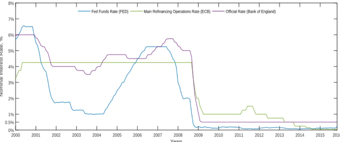
the ECB and the Bank of England, decreased the short-term nominal interest rates
from 5-6% in 2008 to almost 0% in 2014 (see figure 1). Despite these significant drops
in the nominal interest rate, the situation demanded further steps to have a stronger
stimulus, since economies were not reacting to these - hight unemployment rates and
poor economic performance persisted. Hofmann & Bogdanova (2012) showed that
the Taylor rule recommended a negative nominal interest for the advanced economies
around minus 3%2, in order to achieve a desired recovery. However, monetary policy
measures are limited by the non-negativity constraint of the nominal interest rate,
which prevents it to be set below zero. This is commonly known as the zero lower
bound problem (ZLB) of the interest rate channel.
Years
2000 2001 2002 2003 2004 2005 2006 2007 2008 2009 2010 2011 2012 2013 2014 2015 2016
Nominal Interest Rate, %
0% 0.5% 1% 2% 3% 4% 5% 6% 7% 8%
Fed Funds Rate (FED) Main Refinancing Operations Rate (ECB) Official Rate (Bank of England)
Figure 1: The problem of the zero lower bound implicit by the low levels of the
interest rates of the US Fed, ECB and Bank of England.
In normal times the inflation would be expected to be near the target, which is
2
broadly set at 2%. With inflation around this level, policy makers would have the
capacity to change interest rates when necessary without the imminent threat of the
ZLB become binding. However, lately among the developed economies inflation has
been at low levels, which increased the probability of reaching the ZLB and reduced
the capacity of central banks to counteract economic slowdowns.
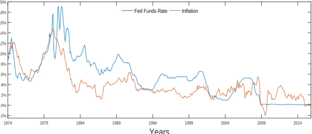
Empirical data for the US from 1974 to 2014 shows that the correlation between
inflation and nominal interest rates is high (the correlation coefficient is 0.74). Figure
2 illustrates this relationship. We can see that, typically, changes in the inflation
tend to be followed by similar changes in the nominal interest rate. This relation is
broken only when the ZLB becomes binding, as we can see in the period from 2009
onwards.
Years
1974 1979 1984 1989 1994 1999 2004 2009 2014 -2%
0% 2% 4% 6% 8% 10% 12% 14% 16% 18% 20%
Fed Funds Rate Inflation
Figure 2: Correlation between the nominal interest rate and inflation rate in the
US from 1974 to 2014. To calculate the inflation we used the data on the consumer price index for all consumers, and all goods.
Thus, admitting that higher average levels of inflation would be followed by higher
average levels of nominal interest rates, increasing the inflation target could decrease
the probability of reaching the ZLB and increase the room for monetary policy to
counteract in those economic slowdowns. Some economists, such as Blanchard et
al (2010), Fuhrer & Madigan (1997) and Reifschneider & Williams (2000), use this
argument to support the idea of increasing the inflation target.
increas-ing the inflation target allows central banks to further reduce the real interest rate
when they decrease the nominal interest rate.
In addition to this action, central banks can use the money supply channel to
boost the economy, which is a good alternative when facing the zero bound. After
unsuccessfully lowering the interest rates, they started a massive program of buying
assets to increase the general liquidity of the economy, known as the quantitative
easing (QE)3. Nonetheless, in this study we will discuss monetary policy in terms
of changes in interest rates rather than in changes in money supply, because it has
become more usual for central banks to use this channel rather than the money
supply channel (see Alvarez et al (2009)).
Using a general equilibrium model, where agents differ in their amount of money
holdings because of the limited access to financial markets, it will be compared the
effect of an unanticipated temporary decrease in the nominal interest rate on the
real interest rate, in three inflation regimes. For this purpose, we will consider the
case of 1%, 2% and 4% inflation. We consider the first case because the average
inflation in the last two years in the US has been 1%. The second case because it
is the actual target. The third is the one suggested by Blanchard et al (2010) and
Fuhrer & Madigan (1997).
We use an inventory-theoretic model of money demand for two reasons. On the
one hand, to compare the results of this type of models to the ones used in other
papers, such as in Fuhrer & Madigan (1997) and Reifschneider & Williams (2000).
In this sense, we aim to study how robust are their results. On the other hand, due
to the fact that there is no significant literature using this kind of models to test
their results for different inflation regimes.
This paper is organized as follows. The next section is a literature review. In
section 3 we characterize the economy and the agents (households, firms and the
government). In section 4 we present the conditions for the competitive equilibrium.
3
In section 5 we calibrate the model and present the competitive equilibrium results,
and compare the effects of different levels of inflation targets in the equilibrium
conditions. At the end of the aforementioned section, we will study the effects of
the interest rate shock under different inflation regimes, and in the cases when there
is also a shock in the productivity and when there is not. In section 6 we will present
the main conclusions of our study.
2
Literature Review
The model used in this paper is well-known in the literature. Baumol (1952)
and Tobin (1956) both used an inventory theoretic model of money demand in
which the market for consumption goods and for financial assets was segmented.
The existence of transaction costs makes agents trade funds between each market
infrequently. As such, they hold inventories of money to pay their consumption
until the next transfer. Romer (1986) has also used this type of models to study the
effects of inflation on capital stock accumulation and money demand elasticity.
In order to have real effects, changes in the nominal interest rate should not be
accompanied by one-to-one opposite changes in the inflation rate, because in that
case the real rate would remain unchanged. To better understand this reasoning, it
is useful to use the Fischer equation to decompose the change in the real interest
rate in two parts: the change in the nominal interest rate and the change in the
expected inflation rate. The equation can be written as r ≈ i−πe, where r is the
real interest rate,i is the nominal interest rate and πe is the expected inflation. In
other words, prices must adjust sluggishly to changes in the nominal interest rate.
However, there can be various reasons for such sluggish adjustment.
Grossman & Weiss (1983) and Rotemberg (1984) have used this setup to
anal-yse the effects of expansionary open market operations (OMO) in i and r. They
prices, but because people tend to spend that extra money smoothly throughout
the period (sluggish expenditure). As such, prices increase only gradually. For this
reason, in order for either OMO or direct changes ini to have real effects it should
be the case that there are or nominal rigidities (the typical Keynesian scheme) or
households have inventories of money (Baumol-Tobin scheme).
Fuhrer & Madigan (1997) and Orphanides & Wieland (1998) studied how the
effectiveness of monetary policy changes as the target of inflation changes. It is
unanimous among the authors that if the inflation target is lower, then the
prob-ability of the zero bound becomes binding increases. In fact, Fuhrer & Madigan
(1997) claimed that central banks might not be able to invert the cycle if the
short-term nominal interest rates are already close to zero due to low inflation level. The
results of Orphanides & Wieland (1998) go in line with the general idea of our work,
i.e., increasing inflation target increases the monetary policy effectiveness, namely
by allowing a bigger fall in the interest rate, which prevents the output gap from
being higher during recessions.
The model used in this work will be similar to the one used by Alvarez et al (2009)
and Verheij (2012). We will construct a cash-in-advance model with exogenous
market segmentation. This means that, in practice, no transfer costs will be charged
to households, contrasting with Alvarez et al (2002), Alvarez & Lippi (2011) and
Silva (2012), but instead we will impose a timing between each transfer (households
can only transfer funds between each account everyN >1).
One important conclusion of Alvarez et al (2009) is that, in a setup where prices
are flexible, inflation responds sluggishly to an exogenous increase in the nominal
interest rate. This means that the model used is able to produce real effects in the
interest rate. An important feature sustaining these results is the endogeneity of
the velocity of money, V, which goes in line with the sluggish expenditure response
of agents found by Grossman & Weiss (1983) and Rotemberg (1984). Making V
a higher V when the inflation is higher than otherwise because when the inflation
is higher, so it is the interest rate level. If this happens, then the money demand
decreases, and so the velocity of money increases (see also Mendiz´abal (2006)).
Since our model will test different steady state inflation regimes, it must be taken
into account that the number of times agents go to the bank is different in each
one. As noticed by Jovanovic (1982), if inflation increases, then the number of
times agents go to the bank increases, and so the holding period decreases (the time
between each trip). This happens because agents have less amounts of money (due
to higher interest rates). Thus, our model will have different holding periods for
each different level of inflation (in part 5.1 we discuss this issue in a more detailed
way).
Moreover, this work will be different from that of previous authors because while
it will be applied an exogenous shock in the nominal interest rate over different
levels of inflation, and then study the reaction of the real interest rate (r), inflation (π) and output (Y), they did this shock considering the same steady-state level of inflation. Besides, we will include the negative productivity shock in a second case,
as in Benk (2005) and Cooley & Hansen (1989).
Unlike Alvarez et al (2009), we make the production endogenous (as in Verheij
(2012)) and allow the productivity factor to vary under specific circumstances. We
also contrast the representative agent models of Fuhrer & Madigan (1997) and
Or-phanides & Wieland (1998), since the source of frictions is the fact that not all
agents are participating in the market at the same time, so they are heterogeneous
3
Model
3.1
Households
There will exist infinitely lived households and each one is composed by a worker,
a shopper and an entrepreneur. The worker supplies units of labour to firms, the
shopper purchases consumption goods and the entrepreneur is who trades bonds. As
in the standard cash-in-advance models, each period is divided into two sub periods
and each market opens at different sub-periods. In the first sub-period, the financial
market opens and the entrepreneur trades bonds using the financial account. In the
second, the goods market opens and the shopper purchases consumption goods,
which can only be purchased using money held in the bank account.
Households can only transfer funds between each account everyN >1 periods -if N = 1 then the model would be reduced to the standard cash-in-advance model, in which agents could transfer funds between each account every period. As this
assumption is exogenously imposed, they will have inventories of money in their
bank account high enough to pay their consumption throughout the time period in
which they cannot make a transfer.
Time is discrete and denoted by t = 1,2, . . . and only a constant fraction 1/N
of households will be active each period. For simplicity, as in Silva (2012), Alvarez
et al (2009) and Verheij (2012), household s will make a transaction at t = Tj(s),
j = 0,1,2, ....
As only a fraction of households is active each period, they face a restriction on
the number of times they can transfer funds between the each account. If they are
active at timet, then they can transfer funds between the two accounts. Let us call this nominal transferXt(s). If not, they can only purchase consumption goods using
the money they hold since the last time they did a transaction. Letptct(s) denote
that nominal expenditure. Each worker earns Wtht(s) from his labour, where Wt
They pay lump-sum taxes as well, denoted by σt. Let γ ∈ [0,1] be the paycheck
parameter as in Alvarez et al (2009), in which γ denotes the percentage of labour earnings that is deposited in the bank account, and 1−γ in the financial account.
Each household s has to satisfy the inter-temporal budget constraint and the constraints in both accounts. First we present the constraint of both accounts
and after the inter-temporal budget constraint that will be used in the household’s
maximization problem.
The sequence of the bank account constraint is derived as follows. If the household
is not active at t, so t 6= Tj(s), then the quantity of money it holds at that time
is restricted to the unspent money from the previous period, Zt−1(s), and to theγ
part of his last period earnings, γWt−1ht−1(s). On the other hand, if the household
s is active at time t, so t = Tj(s), then it can transfer funds from the financial
account to the bank account. Therefore, the constraint on the financial account for
a households is,
Mt(s) = Zt−1(s) +γWt−1ht−1(s), t6=Tj(s) (1)
Mt(s) = Zt−1(s) +γWt−1ht−1(s) +Xt(s), t=Tj(s) (2)
The cash-in-advance constraint of the bank account restricts the consumption
expenditure and the amount of money carried on from the previous period to be
bounded by the amount of money the households has (3). Moreover, Zt(s) ≥ 0,
meaning that households can not borrow money.
ptct(s) +Zt(s)≤Mt(s) (3)
Now we move to the financial account constraint. Households can use the financial
account to trade one-period risk-free non-contingent bonds,Bt(s), with price equal
rate, which is deposited in the financial account in the next period. Moreover, each
period the financial account will be credited by (1−γ)Wt−1ht−1(s) and debited by
the amount of taxes, σt−1. Therefore, the constraint on the bank account for a
household s is,
Bt(s)6(1−γ)Wt−1ht−1(s) + (1 +it−1)Bt−1(s)−σt, t6=Tj(s) (4)
Bt(s)6(1−γ)Wt−1ht−1(s) + (1 +it−1)Bt−1(s)−Xt(s)−σt, t=Tj(s) (5)
Now we turn to the sequence of the inter-temporal budget constraint. At the
beginning of periodt each household has to decide the amount of money and bonds it desires to hold, subject to its level of wealth at that period,
Mt(s) +Bt(s)≤Wt(s) (6)
The wealth at the beginning of each periodtwill depend on the payments received by the hours of labour supplied in the previous period, Wt−1ht−1(s), the unspent
money of the same previous period, Zt−1(s), the interest received on bonds, (1 +
it−1)Bt−1(s) and the amount of taxes paid in the previous period, σt−1. Therefore,
the wealth for each period can be written as4,
Wt(s) = Wt−1ht−1(s) +Zt−1(s) + (1 +it−1)Bt−1(s)−σt−1 (7)
If we substitute (7) in (6) we get the period by period budget constraint. If we
sum fromt= 0,1,2, . . . and multiply byQt=
1
(1 +i0)×...×(1 +it)
, withQ0 = 1,
such that households make the decision at time 0, we get the present value of the
4
The expression for the nominal wealth comes from the restrictions (1), (2), (4) and (5). Note that Xt(s) is not wealth because it is just a transfer between the two accounts. For this reason,
inter-temporal budget constraint of household s,
∞ X
t=0
Qt(s)Mt(s)6W0+
∞ X
t=0
Qt+1(s)Wtht(s) +
∞ X
t=0
Qt+1(s)Zt(s)−
∞ X
t=0
Qt+1σt(s) (8)
W0 is the exogenous initial nominal wealth of household s in terms of money, ¯
M0 >0, and bonds, ¯B0 >0.
Following the developments of previous authors, such as Verheij (2012) and Silva
(2012), we now look at the cash-in-advance constraint of households between each
holding period, i.e., the period of time between each transfer - Tj+1(s) and Tj(s),
j = 0,1,2, . . .. In the first holding period, the household’s expenditures will depend on the initial exogenous money holdings, ¯M0, and on the earnings from labour
of that period. However, the constraint for the first holding period, between t = [T0(s), T1(s)−1], will be different from that of the sequent holding periods, forj ≥1,
because the amount of money available in the first holding period do not depend
on the agent choices, so it can be optimal, given his pattern of consumption, not to
spend all the money. As such,Zt−1(s) might be positive, for t=T1(s)−1.
However, one should have in mind that for the sequent holding periods the amount
of unspent money that is carried to the next period is zero because it is not optimal.
The reason is the fact that as long as the interest rate is positive, the agent is
losing interest. This way, he will only have in the bank account exactly the quantity
enough to pay the consumption. Thus, the holding period cash-in-advance constraint
is given by,
pTj(s)cTj(s)(s) +· · ·+pTj+1(s)−1cTj+1(s)−1(s) +ZT1(s)−1
6M¯0+γ(WTj(s)hTj(s)+· · ·+WTj+1(s)−2hTj+1(s)−2), j = 0,1,2, ...
(9)
Now that we have described the sequence of cash-in-advance constraint we can
introduce it into the inter-temporal budget constraint derived earlier (8). Doing this,
problem, which is equal to the one used in Verheij (2012)5,
∞ X
j=0
QTj
Tj+1(s)−1
X
t=Tj(s)
ptct(s)6φ+
∞ X
j=0
QTj(s)
Tj+1(s)−2
X
t=Tj(s)−1
γWtht(s) + (1−γ)
∞ X
t=0
Qt+1Wtht(s)
+ (QT1(s)−1)( ¯M0 +
T1(s)−2
X
t=0
γWtht(s)−
T1(s)−1
X
t=0
ptct(s)) (10)
φ=W0−P∞
t=0Qt+1σt(s).
In each period, agents get utility from consumption,ct, and from leisure, (1−ht).
The period-by-period utility function is the same used in King et al (1988), and
more recently by Verheij (2012) and Silva (2012), since its properties ensure an
equilibrium state,
U(ct(s), ht(s)) =
[ct(s)(1−ht(s))α]1−1/η
1−1/η (11)
The parameters α and 1/η represent the relative preference for leisure and the relative risk aversion, respectively.
The household’s problem consists in choosing the optimal sequence of
consump-tion, {ct(s)}∞t=0, and leisure,{ht(s)}∞t=0, such that its utility function is maximized,
max
∞ X
t=0
βt[ct(s)(1−ht(s))
α]1−1/η
1−1/η (12)
subject to the its inter-temporal budget constraint, (10) and the constraint on the
bank account for the first holding-period6,
T1(s)−1
X
t=0
ptct(s))6M¯0 +
T1(s)−2
X
t=0
γWtht(s) (13)
The parameter β is the discount factor, 0< β <1.
5
See section “Inter-temporal budget constraint” of appendix to see the extended explanation.
6
The first-order conditions are the following:
[ct] : βtUc,t(s) = Pt[λ(s)QT1(s)+µ(s)] M.1 t=T0(s), ..., T1(s)−1
[ct] : βtUc,t(s) = Ptλ(s)QTj(s) M.2
t=Tj(s), ..., Tj+1(s)−1
[ht] : βtUh,t(s) = −Wt{λ(s)[(1−γ)Qt+1+QT1(s)γ] +µ(s)γ} M.3 t=T0(s), ..., T1(s)−2
[ht] : βtUh,t(s) = −Wt{λ(s)[QTj(s)γ+ (1−γ)Qt+1(s)]} M.4
t=Tj(s), ..., Tj+1(s)−2
For simplicity of exposition, we denoteUc,t(s) andUh,t(s) the marginal utilities of
consumption and labour of householdsat timet. As in Verheij (2012), from the first order conditions, we can find inter and intra-holding marginal rate of substitution
of consumption and inter and intra-holding marginal rate of substitution between
leisure and consumption.
The intra-holding marginal rate of substitution of consumption, i.e. in the same
holding period, is the following,
Uc,t(s)
Uc,t+1(s)
= βPt
Pt+1
, t=Tj(s), ..., Tj+1(s)−1 (14)
For any pair hTj(s), Tj+1(s)
i
, j = 1,2,3, ..., the inter-holding marginal rate of substitution of consumption is,
βTj(s)U
c,Tj(s)(s)
βTj+1(s)U
c,Tj+1(s)(s)
= QTj(s)PTj(s)
QTj+1(s)PTj+1(s)
(15)
In the special case of the first and second holding periods, t = T0(s) = 0 and
t=T1(s), the inter-holding marginal rate of substitution depends on the Lagrange
constraint of the first holding period,
Uc,0(s)
P0
= β
T1(s)U
c,T1(s)(s) PT1(s)
"
1 + µ(s)
λ(s)QT1(s)
#
(16)
Following the same reasoning, it will exist four marginal rates of substitution
between leisure and consumption, two for the first holding period and two for the
other periods.
The marginal rate of substitution between leisure and consumption for the first
holding period are,
−Uh,t(s)
Uc,t(s)
= Wt{λt(s)[(1−γ)Qt+1+QT1(s)γ] +µt(s)γ} Pt[λt(s)QT1(s)+µt(s)]
, t=T0(s), ..., T1(s)−2
(17)
−Uh,t(s)
Uc,t(s)
= Wt{µt(s)γ−λt(s)Qt+1}
Pt[λt(s)QT1(s)+µt(s)]
, t=T1(s)−1 (18)
And for the other periods it is,
−Uh,t(s)
Uc,t(s)
= Wt{QTj(s)γ+ (1−γ)Qt+1(s)}
PtQTj(s)
, t=Tj(s), ..., Tj+1(s)−2 (19)
−Uh,t(s)
Uc,t(s)
= Wt{QTj(s)γ+ (1−γ)QTj+1(s)} PtQTj(s)
, t=Tj+1(s)−1 (20)
3.2
Firms
Contrary to the endowment economies in the models of Alvarez et al (2012),
Chiu (2007), amongst others, the production in our model will be endogenous. As
in the case of Silva (2012), Adao & Silva (2012), Verheij (2012), Enders (2015) and
Edmond (2003), firms will operate in perfectly competitive markets and hire labour
supplied by households as the unique input of production. This input is traded in a
The production technology will be given by,
Yt=AtLt (21)
At=ϕaAt−1+ǫt, ǫt ∼N(0, σ2), 0< ϕa <1 (22)
At is the parameter that controls the total factor productivity. Firms will
maxi-mize production subject to,
C(w) = WtLt (23)
From the the firms’ problem, we know that the real remuneration of the
produc-tion factor is equal to its marginal physical productivities,
Wt/Pt=At (24)
3.3
Government
The government issues bonds, ¯Bt, and prints money, ¯Mt. For simplicity, in this
exercise we will not consider public expenditures, and the unique spending will
con-cern the debt service, both interest and debt amortization (as in Alvarez et al (2009)
and Edmond (2003)). Revenues come from taxes, ¯σt, collected from households and
new issued debt, ¯Bt. This way, the period-by-period budget constraint states that
the spending, (1 +it−1) ¯Bt−1, should not be higher than the revenue side,
(1 +it−1) ¯Bt−1 6M¯t−M¯t−1+ ¯Bt+ ¯σt (25)
inter-temporal government budget constraint,
G0 6
∞ X
t=0
Qt+1M¯tit+1+
∞ X
t=1
Qtσ¯t (26)
G0 are the initial public obligations on money and bonds, and P∞
t=0Qt+1M¯tit+1
is the present value of future seigniorage revenues.
4
Stationary Equilibrium
4.1
Competitive Equilibrium
A competitive equilibrium is a collection of allocations{ct(s), ht(s), Mt(s), Bt(s)}∞t=0
and prices{Qt, πt}∞t=0such that households and firms maximize their utility and
pro-duction functions, the government satisfies its budget constraint and markets clear.
The economy will be in equilibrium when the goods market is in equilibrium, 1
N
PN−1
s=0 ct(s) = Yt, the labour is in equilibrium,
1
N
PN−1
s=0 ht(s) = Lt, the bonds
market is in equilibrium, 1
N
PN−1
s=0 Bt(s) = ¯Bt, and the money market is also in
equilibrium, 1
N
PN−1
s=0 Mt(s) = ¯Mt.
4.2
Solving the Model
The equilibrium will be characterized by constant inflation, nominal interest rate
and productivity. As such, the endogenous variables of the model, consumption,
labour, production and the real interest rate will be constant.
As in Alvarez et al. (2009), Silva (2012) and Verheij (2012), from now on
house-holds will be indexed by the number of periods since they made the last transfer,
denoted by s = 0,1,2, ..., N −1. For instance, a household of type s = 0 is active in the current period. A household of type s= 1 was active in the previous period, and one of the type s=N−1 will be active in the next period.
the following relationship in the steady state,
Uc(s)
Uc(s+ 1)
= β
1 +π, s = 0, ..., N −2 (27)
From the inter-holding marginal rate of substitution of consumption (15) we get
the well-known relationship between nominal interest rate and inflation rate,
1
β =
1 +i
1 +π (28)
From the marginal rate of substitution between leisure and consumption we get
the following,
−Uh(s)
Uc(s)
=A[γ+ (1−γ)(1 +i)−(s+1)], s= 0, ..., N −2 (29)
−Uh(s)
Uc(s)
=A(1 +i)−N , s=N −1 (30)
To solve the steady state system of equations we used the N −1 intra-holding optimal conditions of the marginal rate of substitution between leisure and
con-sumption fors= 0, ..., N−2, plus that fors=N−1, the goods market equilibrium condition and the labour market equilibrium condition. This way, we have to solve a
system of 2N+ 1 equations. These 2N+ 1 equations are used to find theN optimal levels of consumption,N−1 optimal labour supply, the equilibrium output and the equilibrium inflation. Thus, we have 2N + 1 unknowns.
The remaining unknowns of the households, Mt(s), Zt(s), Xt(s) and Bt(s) will
be characterized using the conditions (1), (2), (3), (4) and (5). Note that the real
Using (1) and (2), the real money holdings in the steady state will be,
m(0) =z(N −1) +γAh(N −1) +x(0), s= 0 (31)
m(s) = z(s) +γAh(s), s= 1, ..., N −1 (32)
By condition (3), the real unspent money is defined as,
z(0) =m(0)−c(0), s= 0 (33)
z(s) =m(s)−c(s), s= 1, ..., N −1 (34)
The real money transfers are defined using conditions (1), (3) and the fact that
in equilibrium real money supply is constant, i.e., mt−mt−1 = 0. Thus, we have
that,
x(0) =c(N −1)−γAh(N −1), s= 0 (35)
The equations (4) and (5) give us the conditions to solve for bond holdings7. It
can be shown that real bond holdings are given by,
b(0) b(1) · · ·
b(N−1)
=
1 −1/β . . . −1/β
−1/β 1 . . . −1/β
. . . . . . .. . . . .
−1/β −1/β . . . −1/β
−1
(1−γ)Ah(0)−x(0)
(1−γ)Ah(1) . . .
(1−γ)Ah(N−1)
5
Results
5.1
Steady State
5.1.1 Calibration
The model will be calibrated so that it adjusts to the U.S. economy in the period
between 1974 and 2014. The parameters that have to be calibrated are β, α, η, γ,
7
N and A. We will define β, the discount factor, equal to 1 1.03
1/12
, such that 2%
annual inflation implies an annual real interest rate of 3 %. The preference for
leisure parameter,α, will be set to 1.2, such that agents spend around 40 percent of their time working. We setη, the degree of risk aversion, equal to the value usually used in the literature, which is one (some examples are Silva (2012), Ad˜ao & Silva
(2012) and Verheij (2012)). The paycheck parameter, γ, will be setted equal to 0.6, accordingly to the most recent data on the U.S. households8. The technology
parameter, A, will be setted such that the output of the benchmark case (when
π= 2%) is one.
To calibrateN, the duration of the holding period measured in months, we used the formula proposed by Alvarez et al (2009) to define N under the assumption of an exogenous market segmentation. Their formula relates aggregate velocity, ¯v, to
N and γ, as ¯v = 2/[(N+1)(1-γ)]. However, to use it, we must have data on the velocity of money for each level of inflation, in order to find the correspondentN.
Considering the Quantitative Theory of Money (QTM), where P Y = M V, P
is the price level, Y the real output, M the money demand, and V the velocity of money, we can see that the money-income ratio, M
P Y , is equal to the inverse of the
velocity of money, 1
V . We will estimate the relation between the money-income ratio
and the nominal interest rate to find the velocity of money for each level of interest
rates. After this, we use the level of the nominal interest rate which is compatible
with each inflation regime, given the conditions of our model. In the final, we get a
relation between the velocity and the inflation level.
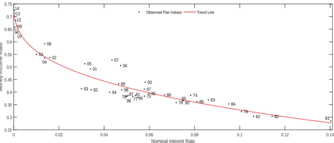
Figure 3 plots the estimates for the relation between the money-income ratio and
the nominal interest rate9. From condition (28), when the inflation level is 1%, 2%
8
As in Alvarez et al (2009) in order to calibrate γ we had to analyse the microeconomic data to see what has been the percentage of the personal income that has been received as wages and salaries of the US households. We observed that this percentage has been around 60% on average over the period from 1974 to 2014. The data was collected from the US National Bureau of Economic Analysis.
9
an 4%, the nominal interest rate is 1.25%, 2.25% and 4.26%, respectively. Then, we
used this values of interest rates to see the corresponding money-income ratio. Our
findings led us to use N equal to 21, 18 and 14 when the inflation is 1%, 2% and
4%, respectively10.
Nominal Interest Rate
0 0.02 0.04 0.06 0.08 0.1 0.12 0.14
Money-Income Ratio 0.25 0.3 0.35 0.4 0.45 0.5 0.55 0.6 0.65 0.7 0.75 74 75 76 77 78 79 80 81 82 83 84 85 86 87 88 89 90 91 92 93 94 95 96 97 98 99 00 01 02 03 04 05 06 07 08 09 10 11 12 13 14
Observed Pair-Values Trend Line
Figure 3: Money-income ratio and nominal interest rates. The curve of
figure 3 is of the type axb +c, with a = −0.9396, b = 0.3233 and c = 0.7751. The
coefficients a, b and c were estimated using the non-linear least squares estimator, with confidence intervals of 95%. These calculations were made using the curve fittingtool in MATLAB. The nominal interest rate is the 3-month treasury bill rate.
Nonetheless, if one were to use the calibration suggested by some authors such as
Silva (2012), where the segmentation is endogenous, N would not be very different from these values. It would be 24, 21 and 18 for 1%, 2% and 4% inflation rate,
respectively.
5.1.2 The Benchmark Case
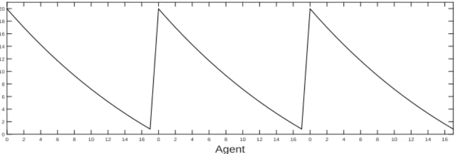
To facilitate the exposition, the case of 2% inflation will be considered the
bench-mark case. Figure 4 shows the typical saw-tooth pattern of money holdings in this
type of model. As we can see, the pattern of the real money holdings is decreasing
as the agent is closer to the transaction moment (which occurs whenN = 18). This happens because the amount they have in the bank account must be sufficient to
Also Lucas and Nicolini (2015) used a new aggregate, the “NewM1”.
10
pay their consumption expenditures throughout the holding period. As such, they
have incentives to spend it steadily.
Given the decreasing pattern of money holdings, their consumption is decreasing
as well, since money is the only good which can be used to pay consumption (figure
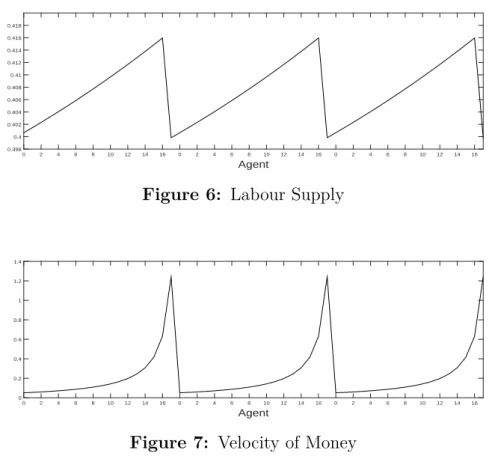
5). Figure 6 shows us the labour supply curve. As we can see, it is increasing ins,
i.e. as the time of the transaction gets closer the labour supplied is higher - as in
the case of the velocity. This fact is expressed in the marginal rate of substitution
between consumption and labour (equations 29 and 30) - whenever consumption is
decreasing, labour supply is increasing.
Agent
0 2 4 6 8 10 12 14 16 0 2 4 6 8 10 12 14 16 0 2 4 6 8 10 12 14 16 0
2 4 6 8 10 12 14 16 18 20
Figure 4: Real Money Holdings
Agent
0 2 4 6 8 10 12 14 16 0 2 4 6 8 10 12 14 16 0 2 4 6 8 10 12 14 16 0.8
0.85 0.9 0.95 1 1.05 1.1 1.15 1.2 1.25
Figure 5: Real Consumption
Figure 7 shows the pattern of the velocity of money. As we can see, it shows
must be sufficient to pay the consumption expenditures until the next transfer. The
non-constant velocity is a characteristic of this type of models.
Note that each household has the same wealth, i.e. Wt(s) is equal for the house-hold of type s = 0 and for the type s = N −1. What differs is how this wealth is split between money and bonds. A household of type s = 0 holds more money and less amount of bonds compared to one of the types=N −1, which holds less money but more bonds. Therefore, while money holdings are decreasing ins, bond holdings are increasing in s, such that the level of wealth remains unchanged.
Agent
0 2 4 6 8 10 12 14 16 0 2 4 6 8 10 12 14 16 0 2 4 6 8 10 12 14 16 0.398
0.4 0.402 0.404 0.406 0.408 0.41 0.412 0.414 0.416 0.418
Figure 6: Labour Supply
Agent
0 2 4 6 8 10 12 14 16 0 2 4 6 8 10 12 14 16 0 2 4 6 8 10 12 14 16 0
0.2 0.4 0.6 0.8 1 1.2 1.4
Figure 7: Velocity of Money
5.1.3 Long Run Implications of Different Inflation Regimes
Before studying the short-run effects of changing the inflation regime, we take a
brief look on what happens in the economy in the long-run. Changing the average
level of inflation makes agents readjust their choices on how to use their money.
future consumption. Thus, money holdings, consumption, labour supply and bond
holdings will change in response to these readjustments.
Agent
0 1 2 3 4 5 6 7 8 9 10 11 12 13 14 15 16 17 18 19 0
5 10 15 20 25
1% Inflation 2% Inflation 4% Inflation
Figure 8: Real Money Holdings
Agent
0 1 2 3 4 5 6 7 8 9 10 11 12 13 14 15 16 17 18 19 20 0.6
0.7 0.8 0.9 1 1.1 1.2 1.3
1% Inflation 2% Inflation 4% Inflation
Figure 9: Real Consumption
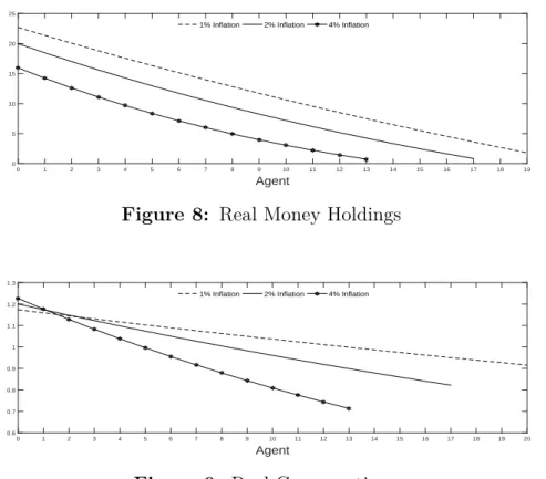
The level of real money holdings decreases as the inflation level increases (figure
8). This happens because rational agents choose to hold less money today and invest
more in bonds today (their bond holdings increases), in order to consume relatively
more in the future, due to the higher nominal interest rates income. In other words,
they choose to postpone a part of their actual level of consumption (figure 9). In
fact, for the majority of the different types of households, the level of consumption
decreases.
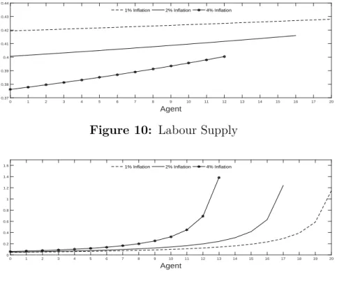
Velocity increases as a result of the fact that the effect of inflation is higher in the
money holdings than in the level of consumption (figure 11). Hence, if the decrease
in the amount of money held is higher than the decrease of present consumption,
velocity increases (also described by Edmond(2003)). Figure 10 plots the changes in
the labour supply. We can see that when the inflation target increases, the amount
Agent
0 1 2 3 4 5 6 7 8 9 10 11 12 13 14 15 16 17 20 0.37
0.38 0.39 0.4 0.41 0.42 0.43 0.44
1% Inflation 2% Inflation 4% Inflation
Figure 10: Labour Supply
Agent
0 1 2 3 4 5 6 7 8 9 10 11 12 13 14 15 16 17 18 19 20 0
0.2 0.4 0.6 0.8 1 1.2 1.4
1.6 1% Inflation 2% Inflation 4% Inflation
Figure 11: Velocity of Money
wages do not adjust to the level of inflation. Another reason pointed by Cooley &
Hansen (1989) is that households increase the consumption of leisure and decrease
the consumption of goods due to the inflation tax charged in the latter. Thus, the
labour supply decreases as the inflation level (and so theinflation tax) increases.
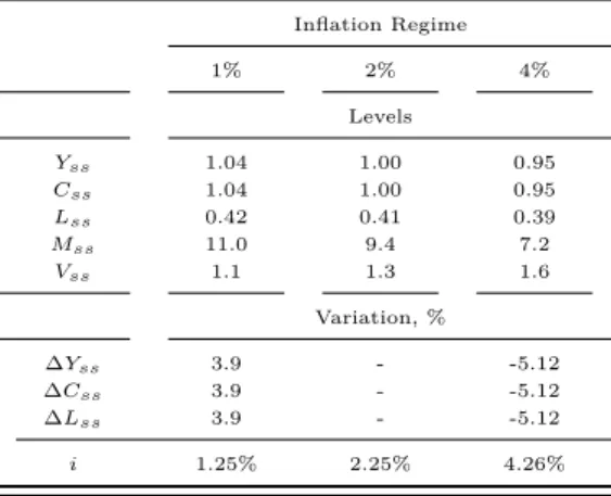
Table 1 summarizes the effects of different levels of inflation on steady state real
output Yss, consumption Css, labour supply Lss, money holdings Mss and velocity
Vss11. The deviations are in respect to the benchmark model (when π∗ = 2%).
One can observe that whenever changes in inflation take place, either positive
or negative, all the variables change. When we increase the average level of
infla-tion producinfla-tion, labour supply and money held by households decreases. On the
opposite, velocity and bond holdings increases (results are very similar to the ones
obtained by Cooley & Hansen (1989)). We can also see that money holdings are more
sensible to changes in inflation than the output. This happens due to the response
of the velocity - when money holdings are increasing, the velocity is decreasing, and
11
vice-versa.
Table 1: Long Run Impact of Changing Inflation Target
Inflation Regime 1% 2% 4%
Levels
Yss 1.04 1.00 0.95
Css 1.04 1.00 0.95
Lss 0.42 0.41 0.39
Mss 11.0 9.4 7.2
Vss 1.1 1.3 1.6
Variation, %
∆Yss 3.9 - -5.12
∆Css 3.9 - -5.12
∆Lss 3.9 - -5.12 i 1.25% 2.25% 4.26%
The heterogeneity of our model allows us to see the equilibrium response of each
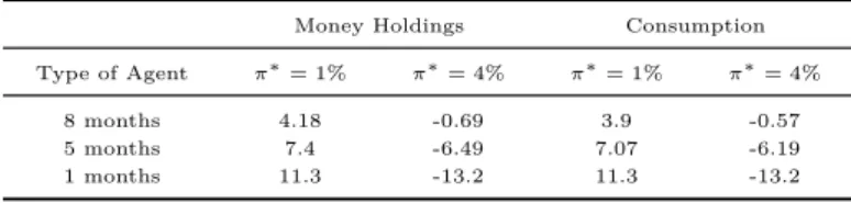
type household to the change in the inflation regime (see table 2)12. For instance,
when the target increases from 2% to 4% the decrease in the money holdings is
increasing in s. This means that those households that will have to wait less time to make a transfer are more willing to give up a higher amount of money than
those that, for instance, have made a transfer in the previous period. Recall that
consumption goods can only be purchased using money. Thus, and given the limit
access households have to their interest income, their money stock has to be sufficient
until the next transfer.
Going from 2% to 1% inflation has similar results, but with different directions.
We have seen that decreasing the inflation, increases the general money holdings.
However, this increase in money holdings is increasing in s. This means that a household of type “5 months” increases less its money holdings compared to one
of the type s = N −1. The reason can be the fact that the first one has made a transfer more recently, and thus it holds a larger amount of money, compared to the
12
types =N −1. Thus, this household has little incentive to have a higher amount of money.
Table 2: Changes to the case π∗ = 2%, %
Money Holdings Consumption Type of Agent π∗= 1% π∗= 4% π∗= 1% π∗= 4%
8 months 4.18 -0.69 3.9 -0.57 5 months 7.4 -6.49 7.07 -6.19 1 months 11.3 -13.2 11.3 -13.2
5.2
Impulse Response Dynamic
5.2.1 Methodology
The model will be solved using non-linear methods using the function fsolve of
MATLAB. First, we assume that after the exogenous shock in the nominal interest
rate the economy will be back to its steady state equilibrium after a sufficient number
of months,t∗. We will assume that both the interest rate and the productivity shock
follows a first-order autoregressive process (AR(1)), and therefore their path are
known. Since both paths are known we can solve the model backwards, i.e., we find
the values for consumption, inflation, hours of labour and production att =t∗−1
using the values at t∗ - note that at t=t∗ the economy is in equilibrium. There is
one value for the equilibrium output, one equilibrium value for the inflation, and N
equilibrium values for consumption and hours of work - since we have defined the
existence of N agents. Therefore there are 2N+2 unknowns. To solve this we need
to use the optimality conditions we have derived earlier: the N −1 intra-holding optimal conditions between t∗ and t=t∗ −1,
Uc,t∗−1(s)
Uc,t∗(s+ 1)
= β
1 +πt∗
The inter-holding optimal condition,
Uc,t∗−1(N −1)
Uc,t∗(0)
= β
1 +πt∗
h
(1 +it∗−N). . .(1 +it∗−1)
i
, s= 0, ..., N −2 (37)
N marginal rate of substitutions between leisure and consumption att=t∗ −1,
−Uh,t∗−1(s)
Uc,t∗−1(s)
=At
"
γ + (1−γ)
(1 +it∗−1−s). . .(1 +it∗−1)
#
, s= 0, ..., N −2 (38)
−Uh,t∗−1(s)
Uc,t∗−1(s)
= At
(1 +it∗−N). . .(1 +it∗−1)
, s=N −1 (39)
The market clearing condition for the goods market,
1
N
N−1
X
s=0
ct∗−1(s) =Yt∗−1 (40)
And the market clearing condition for the labour market,
1
N
N−1
X
s=0
ht∗−1(s) = Lt∗−1 (41)
Summing up, we have to solve a system of 2N+2 equations to find the 2N+2 unknowns. Now that we have the values of inflation, consumption, hours of work
and production we can apply the same method, using the same equations, to solve
fort =t∗−2, and so on.
However, for the first N −1 months there are some households which will be in their first holding period. As we have seen before, for the first holding period
theinter-holding optimal conditions and the marginal rate of substitution of leisure
and consumption depend on the ratio of the Lagrange multipliers (see 16, 17 and
18). Note that, as mentioned by Verheij (2012), the household which is of the type
N −1 additional equations. These equations are the bank account constraints for the N −1 households that are in the first holding period (see 13).
Then, our system of equations become: theN−1intra-holdingoptimal conditions betweent and t=t+ 1, for t= 0,1, ..., N −2
Uc,t(s)
Uc,t+1(s+ 1)
= β
1 +πt
, s= 0, ..., N −2 (42)
The inter-holding optimal condition between t and t+ 1,
Uc,t(N −1)
Uc,t+1(0)
= β
1 +πt+1
"
1 + µ(s)
λ(s)Qt+1
#
, s= 0, ..., N −2 (43)
N marginal rate of substitutions between leisure and consumption at t, if the household has made a first transaction,
−Uh,t(s)
Uc,t(s)
=At
"
γ+ (1−γ)
(1 +it∗−1−s). . .(1 +it∗−1)
#
, s= 0, ..., N −2 (44)
if the household has not yet made a transaction at t,
−Uh,t(s)
Uc,t(s)
=At
{λt(s)[(1−γ)Qt+1+Qt+N−sγ] +µt(s)γ}
[λt(s)Qt+N−s+µt(s)]
, s= 0, ..., N −2 (45)
−Uh,t(s)
Uc,t(s)
=At
{µt(s)γ−λt(s)Qt+1}
[λt(s)Qt+N−s+µt(s)]
(46)
The market clearing condition for the goods market at t, for t= 0,1, . . . , N −2,
1
N
N−1
X
s=0
ct(s) =Yt (47)
The market clearing condition for the labour market att, for t = 0,1, . . . , N−2,
1
N
N−1
X
s=0
And the bank account constraint fort, fort= 0,1, . . . , N −2,
T1(s)−1
X
t=0
ptct(s)6M¯0 +
T1(s)−2
X
t=0
γWtht(s) (49)
For simplicity all equations will be solved assuming they hold with equality. This
means that in practice consumers will not leave any money available in their bank
account from one holding period to the another. As this exercise will be done
using the interest rate channel, as Alvarez et al (2009) pointed out, this creates
an indeterminacy because there are more than just one path of the money growth
which is consistent with an exogenous path of the nominal interest rate (present in
the bank account constraint). Since the empirical results show that, on impact, the
change of the inflation is little or absent (see Christiano et al (1998)) we solve this
choosing the path of the money growth that remains inflation constant in the first
period after the shock (as in Alvarez et al (2009) and Verheij (2012)).
5.2.2 Nominal Interest Rate Shock
As previously stated we intend to study how does the inflation regime influence
the effectiveness of the nominal interest channel used by the monetary authorities
to stimulate the economy. To study this, we will observe what are the responses of
real rates and production to an unanticipated persistent temporary shock of
one-percentage-point in the nominal interest rate. The nominal rate is assumed to follow
an AR(1) process with a persistence coefficient, ρ, equal to 0.87 as in Alvarez et al (2009).
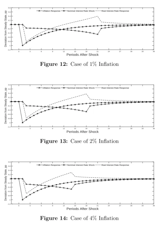
Changing the inflation regime has effects on the real rate adjustment to a shock
in the nominal interest rate. The model used suggests that as the average level of
inflation increases, the response of the real interest rate to that shock is smaller.
This response is measured as deviations from its steady state level, in
impact, the real rate falls by 0.82 pp as a response to a temporary decrease of the
nominal rate of 1 pp, while in the case of 2% and 4% this immediate effect is 0.76
pp and 0.70 pp.
Periods After Shock
0 3 6 9 12 15 18 21 24 27 30 33 36
Deviation from Steady State, pp
-1.2 -1 -0.8 -0.6 -0.4 -0.2 0 0.2 0.4 0.6 0.8
Inflation Response Nominal Interest Rate Shock Real Interest Rate Response
Figure 12: Case of 1% Inflation
Periods After Shock
0 3 6 9 12 15 18 21 24 27 30 33 36
Deviation from Steady State, pp
-1.2 -1 -0.8 -0.6 -0.4 -0.2 0 0.2 0.4 0.6 0.8
Inflation Response Nominal Interest Rate Shock Real Interest Rate Response
Figure 13: Case of 2% Inflation
Periods After Shock
0 3 6 9 12 15 18 21 24 27 30 33 36
Deviation from Steady State, pp
-1.2 -1 -0.8 -0.6 -0.4 -0.2 0 0.2 0.4 0.6 0.8
Inflation Response Nominal Interest Rate Shock Real Interest Rate Response
Figure 14: Case of 4% Inflation
The same figures allows us to see the reason why real rates do not stay constant
when nominal rate changes. The reason is the fact that inflation adjusts sluggishly
to the shock in the nominal interest rate, which allows the real interest rate to vary
thing occur, it would have to be the case that, on impact, the inflation rate increased
by 1pp.
Both inflation and real rate responses produced by the model have different
pat-terns from those presented by homogeneous agent models. This occurs because
every N periods in our model agents readjust their money inventories, increasing the general liquidity of the economy. This could explain why the inflation has the
jump afterN periods - the liquidity of agents could create an inflation pressure. The real rate starts by decreasing as a first result of the shock in the nominal interest.
After this, it stays around 12 months (in the three cases) below its steady state level.
However, as the moment of a new transaction is soon the real rate increases slightly
above its steady state value - but never offsets the immediate fall at the beginning.
In the period after the transaction the real rate drops significantly and then returns
back slowly to its steady state value.
Periods After Shock
0 3 6 9 12 15 18 21 24 27 30 33 36
Deviation from Steady State, pp
-1 -0.8 -0.6 -0.4 -0.2 0 0.2 0.4 0.6 0.8 1
1% Inflation 2% Inflation 4% Inflation
Figure 15: Real Rate Response
Periods After Shock
0 3 6 9 12 15 18 21 24 27 30 33 36
Output Gap, %
-1 -0.5 0 0.5 1 1.5 2 2.5 3
1% Inflation 2% Inflation 4% Inflation
Figure 16: Production Response
Figure 16 shows the evolution of the output after the shock. As expected,
Periods After Shock
0 3 6 9 12 15 18 21 24 27 30 33 36
Deviation from Steady State, pp
-0.8 -0.6 -0.4 -0.2 0 0.2
0.4 1% Inflation 2% Inflation 4% Inflation
Figure 17: Inflation Response
In fact, such interest rate stimulus can increase the production above the potential
at most to around 2%, depending on the inflation level. It seems to be the case that
for higher inflation levels the (positive) output gap is smaller and less long standing.
As we said before, the effects of the increase in the liquidity in the economy have
significant effects on the transition path of the output. As figure 16 suggests, at the
middle of the holding period the output starts to go back to its steady state level.
In the period after the transaction it jumps to 0.8% (around this value in the three
cases) above its steady state level and then the deviation returns slowly to zero.
The reason is that whenever there is a transaction, agents have more money and so
they are able to consume more. This increase in consumption forces the production
to increase. This explains the jump in both output, inflation and real interest rate.
Our model is able to meet the empirical findings about the time monetary policy
measure lag to have their maximum effects on the output. Through figure 16 we
can see that the maximum effect of the monetary policy measure is not reflected in
the output in the first months after it has been applied. It seems to be the case that
the effects of monetary policy in our model have a lag of about 12 to 18 months.
Taylor and Wieland (2012), Batini and Nelson (2002), Gruen et al (1999), Brown
and Santoni (1983) have found empirical evidence that this lag can be between 12
and 24 months.
Figure 17 illustrates the response of inflation for each level of inflation target. It
the pattern of the nominal interest rate, the real rate falls less 13. In other words,
this means that the price stickiness decreases for higher levels of inflation target.
This is somehow connected to the time that agents have to readjust their portfolios
to the shock in the nominal interest rate. Table 3 demonstrates this. For instance,
6 months after the shock in the nominal rate, when the target is 1% the inflation
rate is 0.19 pp below its steady state level, while in the case of a target of 4% it is
0.32 pp below.
Table 3: Degree of price stickiness
Time 1 2 3 4 5 6
π = 1% 0 -0.169 -0.171 -0.176 -0.182 -0.188
π = 2% 0 -0.199 -0.204 -0.211 -0.22 -0.229
π = 4% 0 -0.263 -0.271 -0.283 -0.297 -0.312
Although our model has little uncertainty, the aforementioned fact reflects some
ideas of Friedman (1977). In his paper, the author emphasized the negative effects
of higher levels of inflation on output growth, due to firms’ capacity to extract
information from the market. On empirical grounds, more recently, Judson and
Orphanides (1999) found the same relationship.
5.2.3 The productivity shock
When we add the shock of the productivity factor14 (figure 18), the responses of
the real rate do not change significantly. In the previous case, we noticed that the
real rate fall would be higher, the lower the inflation level. In this case, this relation
is verified again (figure 19). As we can see, the real interest rate declines more, the
lower the average level of inflation15.
13
Our model produced inflation responses such that the higher the target, the higher the volatility of the inflation adjustment. For instance, when the target is 4% the volatility, measured by the standard deviation, is 0.1158, while in the case of 1% is 0.106. Okun (1971) and Caporale et al. (2010), for the Euro Area, have found this empirical relationship as well.
14
We assume that the productivity shock follows an AR(1) process, At = ϕaAt−1+ǫt with a
persistence coefficient,ϕa = 0.95, as in Benk et al (2005) and Cooley & Hansen (1989).
15
Periods After Shock
0 3 6 9 12 15 18 21 24 27 30 33 36 39 42 45 48 51 54 57 60 63 66 69 72 75 78 81 84 87 90 93 96
Deviation from Steady State, pp
-2.5 -2 -1.5 -1 -0.5 0 0.5 1 1.5
Figure 18: Productivity Shock
Periods After Shock
0 3 6 9 12 15 18 21 24 27 30 33 36
Deviation from Steady State, pp
-1.5 -1 -0.5 0 0.5 1
1% Inflation 2% Inflation 4% Inflation
Figure 19: Real Interest Rate Response
However, in this case, when the inflation is equal to 1% and 2%, the real interest
rate falls more when compared to the previous one, due to the response of inflation
- the shock in the productivity, on impact, decreases the production but increases
the consumption, creating a demand-pull inflation. Thus, supporting the previous
relationship, increasing the target would not increase the effectiveness of monetary
policy to invert the business cycle and stimulate the economic activity.
Even when we add a lag between the shock in the productivity and the decrease
of the nominal interest rate, the results do not change16. From our calculations,
only for lags greater than 10 months the results would be different. Since for more
reasonable values, say 3 to 6 months, the results are qualitatively the same, we
assumed the lag to be 0 months.
16
6
Conclusions
Typically when central banks face economic slowdowns they use the interest rate
channel to boost economies. However, we have seen that if the nominal interest
rate is already at low levels, then their capacity to invert such economic slowdowns
is little. The main objective of this dissertation was to study whether increasing
the inflation target could increase the capacity of central banks to invert economic
downturns. Specifically, we aimed to study whether the real interest rate decreases
more when the inflation target is higher, as a response to a negative shock in the
nominal interest rate.
To study this we used a general equilibrium model calibrated to the US economy
for the period between 1974 to 2014. Our model contrasts the results obtained by
Fuhrer & Madigan (1997) and Reifschneider & Williams (2000). It suggests that
increasing the inflation target does not increase the real stimulus of central banks
when they decrease the nominal interest rate by one percentage-point. In fact, the
real interest rate declines more, the lower the target. This applies to both situations,
when the interest rate shock is applied alone and when it occurs at the same time of
the productivity shock. One possible explanation for this is the fact that for higher
levels of inflation targets, the degree of price stickiness is lower. This makes the
response of the real interest rate, on impact, to be smaller.
Another conclusion we can take from the impulse-response data is that our model
is able to match the data on the lag between monetary policy actions and their
maximum effects on the production. On average, the maximum impact is after 15
to 18 months.
What concerns the equilibrium state of the economy, increasing the inflation
target decreases the real money holdings and consumption, since households have
have an incentive to invest more in bonds due to the higher interest rates. But
since the effects of inflation are higher in the money holdings than in their level