MASTER OF SCIENCE IN FINANCE
MASTERS FINAL WORK
DISSERTATION
IMPACT
OF
THE
EU
AND
US
SANCTIONS
ON
THE
FOREIGN
EXCHANGE
RATE
OF
RUSSIA
Dmytro Butuzov
Supervisor:
Paula Cristina Albuquerque
2
Abstract
International economic sanctions became a regular tool to achieve foreign policy
objectives regarding target nation. The sanctions literature mostly focuses on question
whether sanctions succeed their foreign policy goals or not, but not on the damage caused
to the sanctioned economy. The following study attempts to fill this gap by presenting a
theoretical overview of the literature concerning the impact of sanctions on a target
country’s economy. Several studies consider different consequences of sanctions on a target country, such as reduction of investments and international trade. However, this study seeks
to go forward and explore impact on currency exchange rate, which is more substantial
macroeconomic measure of economy than investments and international trade. To be more
precise, the study empirically analyzes the connection between EU and US sanctions and
the foreign exchange rate of Russia, using its monthly data over the period of time from
January 2009 to June 2015.
The findings suggest that implementation of sanctions have a significant negative
impact on the domestic currency value. Moreover, since Ruble is substantially connected
with the oil’s price, the paper tests and confirms the hypothesis that sanctions weaken
3
Table of Contents
1. Introduction 4
2. Economic Impact of Sanctions 5
3. Exchange Rate and Sanctions 9
4. Case Study Sanctions on Russia 12
5. Methodology and Data 17
6. Results and Conclusions 26
4
1. Introduction
Sanctions became popular instrument of foreign policy over the last decade,
especially by United States. Nevertheless, the efficiency of sanctions still remains out of
scope.
While plenty of studies that evaluated effects of sanctions focus on the efficiency of
achieving chosen policy goals on a target nation, it was a small number of studies that
analyzed the impact on a target nation economy. The main and most used type of sanctions
are economic sanctions. They are supposed to lead to deterioration of an economic situation
in the target nation, thereby forcing its government to change certain policy or actions.
Hence, the first thing on which sanction should have an impact is country’s state of
economy, which includes exchange rate, international trade and international investments.
This work seeks to study an impact of sanctions on exchange rate as one of the most
important macro determinants of country’s economy, which is tightly interrelated with
other economic variables.
The paper is organized as follows. Section 2 provides literature review of sanctions
and their impact on economy. Section 3 investigates literature of exchange rate models and
its connection with sanctions. Section 4 lays out the empirical model and specifies the data
5
2. Economic Impact of Sanctions
Economic sanctions are the well-known instruments of diplomacy used to decrease
economic welfare of a target nation, thereby forcing it to follow the interests of
international communities.
Sanctions have never been as popular tools of the foreign policy as nowadays.
Apparently it has led to increase of the scholars’ attention to whether sanctions are effective
or not (Hufbauer et al. 1990; Elliot 1998; Drezner 1999). Even though, the effectiveness is
still questionable. It always depends on the particular cases and circumstances. It could be
reasonable to remember such well-known cases from the last decade as success with the
issue of apartheid in South Africa or fails with nuclear policies of Iran and North Korea.
According to the Hufbauer et al. (2009) most sanctions do not reach their goals.
They appear to be successful only at 34% of cases. It turns out that most successful are
sanctions that are focused on moderate changes of the target country policy. They are
successful in 51% of all cases. And most unsuccessful sanctions are those that try to stop
military intervention. According to the study, only 21% of sanctions’ episodes reached their
goals. Attempts to change regime or increase level of democracy were successful in 31% of
cases.
O’Sullivan (2003) finds that sanctions have bigger chances to be effective if they are multilateral, and they are most likely to fail if sanctions implemented unilaterally.
Drezner (2000), on the other hand, concludes that the chances of success are not
6
Some scientist, such as Hufbauer et al. (1990), Shagabutdinova and Berejikian
(2007), based on pre-1990 episodes, found that financial sanctions appear to be successful
more often than trade sanctions.
Though each case is very particular, there are some unavoidable consequences. For
example, sanctions can lead to an uncertainty that in the meantime increases the risk taken
by the domestic and foreign investors. Thus investment attractiveness of a sanctioned
country is decreasing, that leads to increase of the capital outflow.
Another quite popular topic related to sanctions is so-called “smart sanctions”,
which includes financial sanctions, trade restrictions on particular goods, and travel bans on
key individuals and organizations. The main idea of “smart sanctions” is to harm elite
supporters of the targeted regime, while mass public would not be negatively affected.
Thereby, the elite supporters suppose to suffer from the imposed sanctions and put pressure
upon the targeted government to compromise. According to Drezner (2011),
comprehensive sanctions are more effective than selective measures, however the
superiority of “smart sanctions” is that they minimize humanitarian and human rights
issues. Besides, they do not hamper bilateral trade flows, thereby have minimal cost.
While most of the scholars were paying attention to the efficiency of sanctions only
as success or failure of achieving foreign policy goals, there were some attempts to
breakthrough this tendency.
Hufbauer et al. (1997) were pioneers in researching economic impact of sanctions.
They empirically measured the impact of economic sanctions on bilateral trade flows using
gravity model. They found that economic sanctions have a huge negative impact on
7
(2009) specified that sanctions reduce not only trade between target and sender countries,
but also with all trading partners of a target country. Later on, these findings have been
verified by other scholars such as Yang et al. (2004) and Caruso (2003).
Another important determinant of the country’s economic health that has been
studied in connection with sanctions is foreign investment. Foreign investment is very
powerful tool for economy growth, especially for the developing countries, as they have
low liquidity, and foreign investments are crucial to implement their goals of development.
Biglaiser & Lektzian (2011) studied effect of sanction on Foreign Direct Investment
as the biggest source of foreign capital, using panel data for 171 countries from 1971 to
2000. They found robust evidence that US sanctions significantly decrease US FDI into
target nation due to the high risk and uncertainty.
One more important economic variable is foreign exchange rate which
unfortunately was not studied extensively enough. Foreign exchange rate of the domestic
currency is one of the most crucial macroeconomic determinants that have an influence on
current and future situation of a whole domestic economy’s development and particular economy’s agents. Foreign exchange rate movements have direct impact on the international trade, capital flows, volume of production and consumption, and other
economic and social determinants.
This indicator is more ambiguous than all mentioned above, because the
depreciation of the currency has not only negative consequences, and also the appreciation
has not only positive effects. Increase of a relative currency value makes export less
profitable and more expensive for the international markets, while import turn to be less
8
relative to other currencies makes its export more valuable and potentially makes it cheaper
for the international markets, while import becomes less attractive due to its price growth.
In spite of the fact that cheap currency relative to main trading partners can be
economically profitable, quick exchange rate movements may lead to its high volatility
which according to Arize et al. (2000) would have significant negative effect on the export
flows.
The study from Piana (2001) suggests that devaluation of the domestic currency
increases the country burden of an international debt and provokes large outflows of
interest payments, which can lead to recession effect.
In general, sanctions should harm targeted economy by decreasing foreign
investments and trade, increasing an uncertainty of the country’s political future, which will cause domestic currency depreciation (Sobel, 1998).
9
3. Exchange Rate and Sanctions
Since Bretton Woods system collapsed and floating exchange rate system was
generalized, variety of models were invented trying to explain exchange rate dynamic, as
well as predict its short- and long-term movements.
The most prominent study on structural exchange rate models was made by Meese
and Rogoff (1983). They matched most popular structural models of 1970s against random
walk model on the basis of their out-of-sample forecasting accuracy. The analyzed models
are: the flexible price monetary (Frenkel-Bilson) model, the sticky-price monetary
(Dornbusch-Frankel) model, and the sticky-price asset (Hooper-Morton) model.
Respectively, first model includes money supply, industrial production index and interest
rate. Second model consist all of the mentioned variables plus inflation rate. The third
model includes all of the mentioned variables plus trade balance.
By testing these three models, Meese and Rogoff found that none of these models
can outperform a random walk model at one- to twelve-month horizon for the dollar/pound,
dollar/mark, dollar/yen and the trade-weighted dollar exchange rate. Moreover, after a
number of attempts to argue this statement, evidence to disprove these results were not
found (Rapach and Wohar, 2001; Mark and Sul, 2001).
Nevertheless, Engel et al. (2007) claim that the test based on whether model beats
random walk, is too strong criteria for the model evaluation, because under general
conditions exchange rate movement simulate random walk.
Evans and Lyons (1999) test microstructure model for exchange rate that includes
order flow and interest rate. The model explains more than 50% of JPY/USD and DM/USD
10
macroeconomic fundamentals and microstructure variables to explain US/Jamaica
exchange rate’s movement. The study applies several models and eventually suggests that including micro-based variables improves explanation power for all the models. The paper
finds four statistically significant variables with correct a priori sign for all the models.
These variables are relative money, relative prices, USD purchases and interventions.
Smith (2014) wrote the first paper that seeks to analyze effect of sanction on the
foreign exchange rate using data of 40 countries that were sanctioned by US for some
period between 1976 and 2000. The study considers several models, from which the most
robust one includes gross domestic product, trade balance, foreign reserves, inflation rate
and a dummy for the type of sanctions imposed. Eventually, the model suggests that
comprehensive and financial sanctions have a negative impact on the year changes in
nominal exchange rate.
Another recent paper that is trying to explain the foreign exchange rate was written
by Dreger et al. (2015) studies the case of Russia. The paper is using daily frequency data
of the period from January 2014 to March 2015. The model used in this study includes
nominal exchange rate, oil price, interest rates for overnight loans, sanction indices and
media indices. Sanction index is the composite indicator of sanctions on and from Russia,
which is determined from the cumulative sum of sanction dummies. Media index denotes
of how frequently international media mentions topic related to Russia’s sanctions. The
results of the model conclude that major portion of the Ruble depreciation was caused by
the fall of oil prices, while sanctions have minor positive effect, significant only at the
11
Given the lack of a widely accepted model for nominal exchange rate, especially
with sanctions effect accounted, neither of invented models is likely to be universally
applicable. Therefore, the most reasonable approach is to empirically test various models
12
4. Case Study Sanctions on Russia
Due to the conflict in Ukraine started in 2014, United States, European Union and
some other countries imposed various sanctions on Russia. The first two rounds of
sanctions were travel bans, freezing of assets located in sender countries imposed upon
certain individuals and officials from Russia. It did not have significant effect, neither on
Russia’s policy nor on economy, but definitely caused state of uncertainty, thus making it more vulnerable for the external shocks.
The most crucial package of sanctions was implemented in July 2014, which
imposed restrictions against certain sectors of Russia’s economy. It included restrictions in financial sector, ban on export of military, mining technologies and some engineering
equipment.
Moreover, at the III quarter of 2014 oil price has fallen by 50%, which turns to be a
big loss for the Russia’s economy. According to the U.S. Energy Information Administration, crude oil and petroleum products export accounted for 54% of Russia’s
total export in 2013. Hence, the assessment of the sanctions’ effect is complicated by the
fact that there are two external shocks happened in the short period of time, thus increasing
harmful impact of each other.
As a result, sanctions and the fall of oil price caused huge outflow of the capital,
which led to boost of the volatility on exchange market, depreciation of the Russian
currency by more than 50%, and increase of inflation.
The literature of sanctions mentions several conditions that significantly increase
likelihood of sanctions to be successful. One of the main conditions of successful sanctions
13
instance, sanctions from U.S. on Russia are apparently not as impactful as sanctions from
Europe, given that some of Europe countries are one of the main partners of Russia.
According to the Federal State Statistics Service the major trade partners of Russia
at 2013 were EU countries (27.6% of whole import and 54.7% of whole export), when U.S.
had only 2.3% of export and 3.4% of import. Chart 1 displays import and export with
particular countries in % to whole import and export (based on data from 2014).
Chart 1 – Main trading partners of Russia, %
Source: European Commission Directorate-General Trade’s Statistics
It is important to note that some of the banned U.S. products such as mining
technologies and engineering equipment are unique and licensed, which makes them not
replaceable. And even though, there are no visible consequences for Russia at this point of
time, it may slow down development of new oil and gas fields.
Another condition is that economy of a sender country should be significantly
bigger than economy of a target country, otherwise sanctions will not be successful and
may hurt economy of the sender more than economy of the target (Hufbauer et al., 1990). 0 10 20 30 40 50 60
EU 28 China Turkey Belarus Japan USA
Import Export
14
According to the International Monetary Fund World Economic Outlook from April
2015, Russia holds only 3.1% of the world GDP based on PPP Valuation, whereas U.S.
holds 16.1% and Europe 16.9%. Hence it follows that the economy of Russia significantly
smaller than economy of U.S. or Europe, which increase likelihood of the sanctions to be
successful.
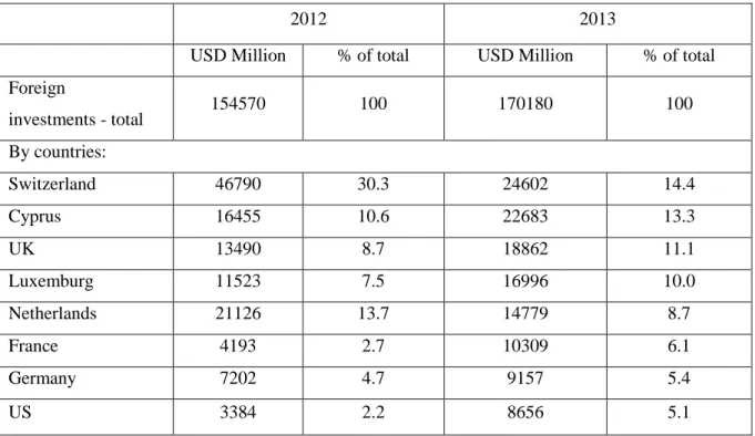
Another measure of partnership importance is the size of its investments. Based on
the Federal State Statistics Service major international investments come from European
Union members. More precisely, in 2013, 46% of import to Russia was from EU countries,
and more than 50% of its export Russia transferred to EU countries. In the meantime,
investments from U.S. accounted for only 5.1%. Table 2 represents inflows of the foreign
investments in Russia at 2012 and 2013.
Table 2 – Inflows of the foreign investments in Russia at 2012 and 2013
2012 2013
USD Million % of total USD Million % of total Foreign investments - total 154570 100 170180 100 By countries: Switzerland 46790 30.3 24602 14.4 Cyprus 16455 10.6 22683 13.3 UK 13490 8.7 18862 11.1 Luxemburg 11523 7.5 16996 10.0 Netherlands 21126 13.7 14779 8.7 France 4193 2.7 10309 6.1 Germany 7202 4.7 9157 5.4 US 3384 2.2 8656 5.1
15
Although US investments are quite small, some sectors of Russia’s economy
significantly rely on U.S. investments such as production of oil products (12% of all
foreign investments in the production of oil products) and production of machines and
equipment (28.1%). Furthermore, several US companies are substantial players in Russia.
For instance, PepsiCo is the largest producer in Russian beverage and food market. Other
examples represent Ford Motor Co., General Electric, Visa and Master Card (Congressional
Research Service).
Paper from Hufbauer et al. (2009) finds level of a target country democracy to be
significant among other explanatory variables. The study finds that the higher the
democracy level, the higher probability of sanctions to achieve stated goals. In accordance
to Polity IV data, Russian Federation has moderately high and stable level of democracy.
The index of Russia is 5 for the scale of indexes from -10 to +10. On the other side, The
Economist Intelligence Unit’s Democracy Index 2015 denotes the Russia’s index as 3.31 for the range from 0 to 10, which puts Russia on 132nd place among 165 countries and defines its regime as authoritarian.
Since this study focuses on exchange rate, it is relevant to briefly consider current
exchange rate regime of Russia. In 2005, the Bank of Russia implemented a dual-currency
basket as main indicator for exchange rate. Then, in 2009 the mechanism of automatic
correction of the allowed boundaries was introduced, according to the amount of
intervention. In 2013, the Bank of Russia started to switch the main tool of managing
exchange rate from interventions to interest rate. In November 2014, the interval of allowed
values of dual-currency basket was finally abolished, as well as necessity for intervention in
16
case of the risk to financial stability. Hence, when the Ruble started to fall in 2014,
significant interventions were made in order to prevent this drop or at least stabilize the
currency. According to the statistics in 2013 the Central bank sold only $24.26 in the
foreign exchange market, but in 2014 CB sold $76.13 billion, from which $11.9 billion
17
5. Methodology and data
The paper investigates the effect of sanction on exchange rate, moreover it seeks to
go further and test the assumption that sanction could interfere relation of exchange rate
and oil price. Hence, the hypotheses that will be tested in this paper are as follows:
H1: The imposition of sanctions on Russia has a negative effect on its domestic
currency versus foreign currencies.
H2: The imposition of sanctions on Russia makes its currency more vulnerable to
external shocks, particularly to the sharp fall of oil price.
Hypothesis 2 assumes that the relation between exchange rate and oil price may
vary due to presence of sanctions, in other words, that sanctions make exchange rate of
Russia more vulnerable to the fall of oil price. Hence, if the hypothesis is true, the relation
between exchange rate and oil price with implemented sanctions is different from when
there are no sanctions. Thus, the study seeks to find weather sanctions made Russia more
vulnerable to external shocks or not. The hypothesis based on the fact that both events
occurred simultaneously, hence it would be misleading not to take into account possible
interference of these two events.
As it is discussed above, there is no widely accepted model for exchange rate.
Thereby, empirical studies use various sets of variables to analyze exchange rate according
to particular characteristics of country. By following this approach, particular structural
model was constructed and adjusted to the economy of Russia. There is a wide range of
18
economic indicators was tested for the relevance, statistically significant impact and
multicollinearity among them. Eventually, the variables chosen for the final model are
money supply, oil price, government interventions, interest rate and sanctions. Apparently,
it is possible to include more variables which will increase the fit of the model, but then it
would decrease the degrees of freedom and statistical power of the regression.
The chosen model specification is denoted as follows:
exrt= f (mt, intervt, oilt, it, dummy) (1)
Money supply (m). Money supply is used as the variable in the most of the models
that seeks to explain exchange rate movements. According to the Flexible Price model
(Frankel, 1976), an increase of money supply leads to depreciation of the national currency.
Sticky Price model (Dornbusch, 1976), also known as Overshooting Model, suggests that
an increase in a country’s money supply reduces domestic interest rate, and then the drop of
interest rate leads to a short-run depreciation of the domestic currency, that is larger than
the long run equilibrium.
Interventions (interv). The purpose of interventions is to stop the drop, or at least to
abate it. In case of Russia, interventions were also used as a tool to keep exchange rate
between determined boundaries.
There have been many controversial results from the impact of interventions on
exchange rate. Nevertheless, Marcel Fratzscher (2005), based on the wide sample of the
major currencies, finds robust evidences of the long-run effect of sterilized interventions on
exchange rate. Moreover, Taylor and Sarno (2001) point out that interventions may have an
impact on foreign exchange markets for a long period as such actions alert other market
19
Oil price (oil). Variety of scholars has studied connection between exchange rates
of commodity-exporting countries to the price of those commodities. Most of them indicate
strong connection between exchange rate and commodities, which in most of the cases is
oil. As reported by Habib and Kalamova (2007) and some other papers, Russian ruble is the
“oil currency”, meaning that world oil price has a strong positive relation with ruble.
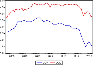
According to Jouko Rautava (2004), oil price has a strong impact on GDP of
Russia. Moreover, simple correlation and variance inflation tests were conducted to check
for the presence of correlation between these two time series. The results indicate strong
correlation, which means that they are highly collinear. Finally, GDP of Russia is presented
only in quarterly frequency, when the rest of the data has monthly frequency. Everything
mentioned above makes GDP inapplicable to use in this study, but fully replaceable by oil
price variable. (Nearly perfect correlation between logarithm of the Brent oil prices and
Russia’s GDP changes in percentage according to the previous period are presented in the attachments section – Figure 1).
Interest rate (i). Raise of interest rate increases potential earnings from investments
in domestic currency, its demand is increasing and thus the currency relative value is also
growing. Central banks widely use interest rate as a tool to stop or relax currency
depreciation. Interest rate is included in all structural and hybrid models.
Descriptive Statistics
Data set is taken from the Data Stream and Federal State Statistic Service. It has
monthly frequency and covers the period from January 2009 to June 2015. The Figures of
all variables are presented in Appendix. The exchange rate is defined as nominal bilateral
20
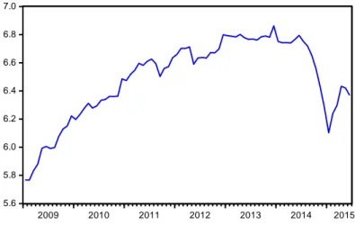
in terms of Ruble (Figure 2). For the money supply variable the M2 measure is used
(Figure 3). Interventions are Russia Central Bank sales of USD (Figure 4). Interest rate is
taken as Russian Interbank middle rate for 31 to 90 days (Figure 5). The oil price variable is
the price of Brent oil in US Dollars per barrel (Figure 6). Sanctions are expressed through
the dummy variable which is equal to 0 until August 2014, when the most substantial
package of sanctions was imposed. The rest of the period dummy is equal to 1, indicating
the presence of sanctions. All the variables are presented in logarithmic form, except the oil
price and dummy variable.
Exchange rate, money supply, interest rate and interventions are taken as
endogenous variables, when oil price, dummy of sanctions and interaction of sanctions with
oil price are taken as exogenous.
Empirical Analysis
The econometric software which is used for employing the tests and constructing the model
is Eviews 8 program.
First of all, Augmented Dickey-Fuller (ADF) Unit Root test was conducted for all
of the variables to check whether they are stationary or not, and if not, what are the orders
21 Table 3. Unit root test.
Time series Level 1st difference
t-Statistics exr 1.25 -3.77* m -2.23 -4.83* interv -1.82 -8.74* i -2.9 -6.73* oil -1.83 -9.06*
Note: The test performed by Augmented Dickey-Fuller (ADF) unit root test. Null hypothesis of the test is presence of a unit root. * denotes rejection of null hypothesis at the 1% significance level. Lag lengths are indicated through Akaike information criterion. Test is performed with a constant.
The paper from Engle and Granger (1987) states, that the linear regression of
non-stationary variables may be non-stationary in case the variables are cointegrated. Vector
Autoregression (VAR) with all endogenous variables is constructed in order to determine
optimal lag length for the Vector Error Correction (VEC) model. On the basis of Schwarz
information criterion two lags are identified as the optimal lag length. Then Johansen
Cointegration test, proposed by Johansen (1988), was performed in order to check for the
presence of long-term relationships among them. Oil price series and dummy are not
included since they are assumed as exogenous variables. Test allows for intercept in
cointegrating equation and VAR. Both versions of the test (Trace and Maximum
Eigenvalue) reject the null hypothesis of no cointegration and indicate presence of 1
22 Table 4. Johansen Cointegration test.
Rank Trace Statistic ME Statistic
0 54.79* (0.0097) 28.28* (0.0407) 1 26.52 (0.114) 19.79 (0.0761) 2 6.72 (0.6102) 6.56 (0.5422) 3 0.002 (0.6893) 0.16 (0.6893)
* denotes rejection of null hypothesis of no cointegration at the 5% significance level. P-values are presented in parentheses.
According to the Lütkepohl et al. (2005), if there are cointegrating relations among
variables, the application of the VAR model will lead to the spurious regression problem.
On the other hand, so-called Vector Error Correction model can be used for the
cointegrating systems. It is restricted version of the VAR model with error correction
features. VEC model enables to describe long- and short-term relationships among
nonstationary time series that are cointegrated in the same order and eliminates the problem
of spurious regression which appears in case of Vector Autoregressive. Hence, Vector Error
Correction model is applied in this study. VEC model estimates cointegration relationship
using Johansen procedure, it also represents speed of adjustment of variables towards long-run equilibrium along with parameters of short-run effect.
Simple form of the VEC model with two cointegrated variables and one lag length
can be presented as follows:
Δxt = λ2 (yt-1 – βxt-1– α) + λ1Δxt-1 + λ2Δyt-1 + εt (2)
Where et-1 = (yt-1 – βxt-1 – α) is so-called error correction term that indicates
23
of disequilibrium, in other words they indicate the response of y and x to deflections from
long-run equilibrium, Δxt-1 and Δyt-1 are the parameters of short-run effect, εt is
independent and identically-distributed error term.
Since specified model has only one cointegrating equation it is also applicable to
run Dynamic Least Squares (DOLS) and Fully Modified Least Squares (FMOLS) models.
As stated in Lyhagen et al. (2007), this restriction occurs since those methods are residual
based. FMOLS and DOLS models correct for endogeneity bias and serial correlation in
cointegrated regression, thus allowing for the standard normal inference.
FMOLS is applying semi-parametric autocorrelation correction using estimated
residuals from cointegrating regressions and differenced explanatory variables. Thus,
FMOLS method adjusts endogeneity and short-term dynamics of the errors (Philips and
Hanson, 1990).
DOLS approach was developed by Saikkonen (1992) and Stock and Watson (1993).
It involves parametric correction for endogeneity by adding lagged values of the first
difference.
𝑥𝑡 = 𝜆0 + 𝜆1𝑍𝑡 + ∑𝑝𝑗=−𝑝𝜆𝑗∆𝑍𝑡−1 + 𝜂𝑡 (3)
Where Zt is a vector of explanatory variables, p is number of lags and Δ is a lag
operator.
At this point, specified regression in VEC, DOLS and FMOLS representations can
be constructed (Table 4). Those models require variables to be first difference stationary,
therefore the variables are taken on the level. All models assume constant as the trend
24
All of the methods indicate stationary long-run relations among exchange rate
(exr), money supply (m), interest rate (i), interventions (interv), price of the oil (oil),
dummy of sanctions (D) and interaction variable (oil*D) with high explanatory power of
each variable and of the whole model. According to the t-statistics, all of the variables are
significant at 1% level of significance.
Table 5. VEC, DOLS and FMOLS models.
Variables VEC DOLS FMOLS Endogenous Variables m 0.3078 (0.0379) [8.1176] 0.2795 (0.047) [5.9482] 0.3333 (0.0570) [5.841] interv 0.000017 (0.000002) [8.1809] 0.000012 (0.0000027) [4.3372] 0.0000039 (0.0000014) [2.721] i 0.0115 (0.0047) [2.4383] 0.0259 (0.0056) [4.6575] 0.0265 (0.0057) [4.6244] Exogenous Variables oil -0.1632 (0.0194) [-8.4333] -0.2419 (0.0577) [-4.1896] -0.3209 (0.0711) [-4.514] D 0.9754 (0.173) [5.6401] 2.3145 (0.3918) [5.9073] 2.1185 (0.4521) [4.6862] oil*D -0.2006 (0.0386) [-5.1949] -0.4887 (0.088) [-5.5528] -0.4453 (0.1005) [-4.4302] R2 Sum sq. residue S.E. equation 0.8687 0.02 0.018 0.9841 0.1953 0.0275 0.9539 0.1953 0.0437
The numbers in ( ) indicate standard errors. T-statistics are presented in [ ].
Test for the inverse roots of the characteristic AR polynomial suggests that the
25
that the number of unit roots has to be equal to the number of endogenous variables minus
the number of cointegrating relationships. At the same time the moduli of the remaining
roots have to be less than unity. Autocorrelation LM test proposed by Johansen (1995)
indicates rejection of serial correlation among residuals since all the p-values are higher
26
6. Results and Conclusion
The coefficients vary considerably between each model. However, VEC, DOLS and
FMOLS approaches denote negative and statistically significant coefficients of the
sanctions variable, which equal to 0.98, 2.31 and 2.12 respectively. Thus, all models
confirm the presence of strong impact of sanctions on exchange rate in the long-run
perspective.
The second hypothesis is that sanctions have substantial influence on the connection
between exchange rate and oil price. VEC, DOLS and FMOLS methods indicate negative
and statistically significant coefficients of 0.2, 0.48 and 0.45 respectively. The results
suggest that the sanctions increase the impact of the world oil price on exchange rate of the
Russian currency.
This paper makes its contribution into a quite unexplored, but very important field
by testing the influence of exchange rate on the relative value of Russia’s domestic
currency and its interference to the relation between the currency and price of the oil. The
study applies exchange rate model based on the literature analysis, but also adjusts it to the
particular case of Russia’s economy. The model is stable and has substantially high explanatory power of the exchange rate movements.
The findings suggest that sanctions are indeed play significant role in exchange rate
value, thus the imposition of sanctions has strong negative effect on the currency’s value.
27
Works Cited
1. Arize, Augustine C., Thomas Osang, and Daniel J. Slottje. "Exchange-rate volatility
and foreign trade: evidence from thirteen LDC's." Journal of Business & Economic
Statistics 18.1 (2000): 10-17.
2. Biglaiser, Glen and David Lektzian. "The effect of sanctions on US foreign direct
investment." International Organization 65.03 (2011): 531-551.
3. Caruso, Raul. "The impact of international economic sanctions on trade: An empirical
analysis." Peace Economics, Peace Science and Public Policy 9.2 (2003).
4. Center for Systemic Peace. Polity IV Project, Political Regime Characteristics and
Transitions. Available from: http://www.systemicpeace.org/inscr/p4v2015.xls (2015).
5. Darby, Julia, Andrew Harlett, Jonathan Ireland and Laura Piscitelli. "The impact of
exchange rate uncertainty on the level of investment." The Economic Journal 109.454
(1999): 55-67.
6. Dornbusch, Rudiger. "Expectations and exchange rate dynamics." The Journal of
Political Economy (1976): 1161-1176.
7. Dreger, Christian, Jarko Fidrmuc, Konstantin Kholodilin and Dirk Ulbricht. "The
Ruble between the hammer and the anvil: Oil prices and economic sanctions." BOFIT
Discussion Paper No. 25/2015 (2015).
8. Drezner, Daniel W. “The sanctions paradox: Economic statecraft and international
relations.” No. 65. Cambridge University Press (1999).
9. Drezner, Daniel W. "Bargaining, enforcement, and multilateral sanctions: when is
28
10. Drezner, Daniel W. "Sanctions sometimes smart: targeted sanctions in theory and
practice." International Studies Review 13.1 (2011): 96-108.
11. Engle, Robert F., and Clive WJ Granger. "Co-integration and error correction:
representation, estimation, and testing." Econometrica: Journal of the Econometric
Society (1987): 251-276.
12. Engel, Charles, Nelson C. Mark, and Kenneth D. West. Exchange rate models are not
as bad as you think. No. w13318. National Bureau of Economic Research (2007).
13. European Commission. European Union, Trade in goods with Russia - Trade Statistics.
Available from:
http://trade.ec.europa.eu/doclib/docs/2006/september/tradoc_113440.pdf (2015).
14. Evans, Martin DD, and Richard K. Lyons. Order flow and exchange rate dynamics.
No. w7317. National Bureau of Economic Research (1999).
15. Foreign investments by the main countries investors. Russia: Federal State Statistics
Service. Available from:
http://www.gks.ru/bgd/regl/b14_13/IssWWW.exe/Stg/d04/24-22.htm (2014).
16. Foreign investments in the economy of Russia. Russia: Federal State Statistics Service.
Available from: http://www.gks.ru/bgd/regl/b14_12/IssWWW.exe/stg/d02/24-10.htm
(2014).
17. Fratzscher, Marcel. "How successful are exchange rate communication and
interventions? Evidence from time-series and event-study approaches." ECB Working
Paper No. 528 (2005).
18. Habib, Maurizio Michael, and Margarita M. Kalamova. "Are there oil currencies? The
29
19. Hufbauer, Gary Clyde, Jeffrey J. Schott, and Kimberly Ann Elliott. Economic
sanctions reconsidered: History and current policy. Vol. 1. Peterson Institute (1990).
20. Hufbauer, Gary Clyde, Kimberly Elliott, Tess Cyrus, Elizabeth Winston "US economic
sanctions: Their impact on trade, jobs, and wages." Institute for International
Economics 3 (1997).
21. Hufbauer, Gary Clyde, Jeffrey J. Schott and Kimberly Elliott, Economic Sanctions
Reconsidered (3rd edition), Washington DC: Peterson institute (2009): 127.
22. Johansen, Søren. "Statistical analysis of cointegration vectors." Journal of Economic
Dynamics and Control 12.2 (1988): 231-254.
23. Johansen, Soren. "Likelihood-based inference in cointegrated vector autoregressive
models." OUP Catalogue (1995).
24. Rautava, Jouko. "The role of oil prices and the real exchange rate in Russia's economy
— a cointegration approach." Journal of Comparative Economics 32.2 (2004): 315-327.
25. Lütkepohl, Helmut. New introduction to multiple time series analysis. Springer
Science & Business Media (2005).
26. Lyhagen, Johan, Pär Österholm, and Mikael Carlsson. Testing for purchasing power
parity in cointegrated panels. No. 7-287. International Monetary Fund (2007).
27. Mark, Nelson C., and Donggyu Sul. "Nominal exchange rates and monetary
fundamentals: evidence from a small post-Bretton Woods panel." Journal of
30
28. McLean, Elena V., and Taehee Whang. "Friends or foes? Major trading partners and
the success of economic sanctions." International Studies Quarterly 54.2 (2010):
427-447.
29. Meese, Richard A., and Kenneth Rogoff. "Empirical exchange rate models of the
seventies: Do they fit out of sample?" Journal of International Economics 14.1 (1983):
3-2.
30. Nelson, Rebeca. U.S.-Russia Economic Relations. Congressional Research Service.
Available from: http://fas.org/sgp/crs/row/IN10119.pdf#_Ref390161120 (2014).
31. O'Sullivan, Meghan L. “Shrewd sanctions: statecraft and state sponsors of terrorism.”
Brookings Institution Press (2003).
32. Phillips, Peter CB, and Bruce E. Hansen. "Statistical inference in instrumental
variables regression with I (1) processes." The Review of Economic Studies 57.1
(1990): 99-125.
33. Piana, Valentino. "Exchange rate." Retrieved April 20 (2001): 2010.
34. Rapach, David E. and Mark E. Wohar. "Testing the monetary model of exchange rate
determination: new evidence from a century of data." Journal of International
Economics 58.2 (2002): 359-385.
35. Saikkonen, Pentti. "Estimation and testing of cointegrated systems by an
autoregressive approximation." Econometric theory 8.01 (1992): 1-27.
36. Shagabutdinova, Ella and Jeffrey Berejikian. "Deploying Sanctions while Protecting
Human Rights: Are Humanitarian “Smart” Sanctions Effective?." Journal of Human Rights 6.1 (2007): 59-74.
31
37. Smith, Matthew U. "What is the effect of US-led sanctions on a target nation's foreign
currency exchange rate?." Georgetown University (2014).
38. Sobel, Russell S. "Exchange rate evidence on the effectiveness of United Nations
policy." Public Choice 95.1 (1998): 1-25.
39. Stock, James H. and Mark W. Watson. "A simple estimator of cointegrating vectors in
higher order integrated systems." Econometrica: Journal of the Econometric
Society (1993): 783-820.
40. Taylor, Mark P. and Lucio Sarno. "Official intervention in the foreign exchange
market: is it effective, and, if so, how does it work?." CEPR Discussion Paper No.
2690 (2001).
41. The Economist Intelligence Unit (2015). Democracy Index 2015: Democracy in an age
of anxiety. Available from:
http://www.eiu.com/public/topical_report.aspx?campaignid=DemocracyIndex2015.
42. U.S. Energy Information Administration (2013). Available from:
http://www.eia.gov/todayinenergy/detail.cfm?id=17231.
43. World Economic Outlook Database. Russia, United States, Europe: International
Monetary Fund. Available from:
http://www.imf.org/external/pubs/ft/weo/2015/01/weodata/index.aspx (July 2015)
44. Wright, Allan S., Roland C. Craigwell, and Diaram RamjeeSingh. "Exchange rate
determination in Jamaica: A market microstructures and macroeconomic fundamentals
approach." MRPA Paper (2007).
45. Yang, Jiawen, Hossein Askari, John Forrer, and Hildy Teegen. "US economic
32
Appendix
Figure 1 – Russia GDP change in percentage according to the previous period and logarithm of the Brent oil price.
1.0 1.5 2.0 2.5 3.0 3.5 4.0 4.5 5.0 2009 2010 2011 2012 2013 2014 2015 GDP LOIL
Figure 2 – Log-transformed time series of the exchange rate variable
3.3 3.4 3.5 3.6 3.7 3.8 3.9 4.0 4.1 4.2 2009 2010 2011 2012 2013 2014 2015
33
Figure 3 – Log-transformed time series of the money supply variable
5.6 5.8 6.0 6.2 6.4 6.6 6.8 7.0 2009 2010 2011 2012 2013 2014 2015
Figure 4 – Log-transformed time series of the intervention variable
0 4,000 8,000 12,000 16,000 20,000 24,000 28,000 2009 2010 2011 2012 2013 2014 2015
Figure 5 – Log-transformed time series of the interest rate variable
4 6 8 10 12 14 16 18 2009 2010 2011 2012 2013 2014 2015
34
Figure 6 – Log-transformed time series of the oil price variable
3.6 3.8 4.0 4.2 4.4 4.6 4.8 5.0 2009 2010 2011 2012 2013 2014 2015