Object detection with artificial vision and neural networks for service robots

Universidade do Minho

Escola de Engenharia

Tiago Alexandre Barbosa Pinto

Object detection with artificial vision and

neural networks for service robots

Universidade do Minho

Escola de Engenharia

Tiago Alexandre Barbosa Pinto

Object detection with artificial vision and

neural networks for service robots

Dissertação de Mestrado em Engenharia Eletrónica

Industrial e Computadores

Trabalho efectuado sob a orientação do

Professor Doutor Agostinho Gil Teixeira Lopes

A

CKNOWLEDGEMENTS

This dissertation ends my cycle of studies concerning the master’s degree and is the culmination of five years of knowledge that was obtained by the academic journey.

This journey was filled with very good colleagues who without them this journey would be very different and teachers who promoted the interest for the subjects.

At first, I would like to thank my adviser, Professor Gil Lopes, for the opportunity of working in a theme that I have always had a lot of interest and a very deep curiosity of working with and for the great provided support and freedom for the development of the dissertation, which it gave me a constant desire to carry it out.

Moreover, I would like to thank my parents who have been relentless in making this possible. Without them I would not be at this turning point. They were the ones who always backed me up in the most difficult times by just being there when I needed the most, always promoting my values and my assets.

A

BSTRACT

This dissertation arises from a major project that consists on developing a domestic service robot, named CHARMIE (Collaborative Home Assistant Robot by Minho Industrial Electronics), to cooperate and help on domestic tasks. In general, the project aims to implement artificial intelligence in the whole robot.

The main contribution of this dissertation is the development of the vision system, with artificial intelligence, to classify and detect, in real time, the objects represented on the environment that the robot is placed.

This dissertation is within two broad areas that revolutionized the robotics industry, namely the artificial vision and artificial intelligence. Knowing that most of the existent information is presented on the vision and with the evolution of robotics, there was a need to introduce the capacity to acquire and process this kind of information. So, the artificial vision algorithms allowed them to acquire information of the environment, namely patterns, objects, formats, through vision sensors (cameras). Although implementing artificial vision can be very complex if it is intended to detect objects, due to image complexity.

The introduction of artificial intelligence, more precisely, deep learning, brought the capability of implementing systems that can learn from provided data, without the need of hard coding it, reducing slightly the complexity and the time consumption of implementing complex problems. For artificial vision problems, like this project, there is a deep neural network that is specialized in learning from three dimensional vectors, namely images, named Convolutional Neural Network (CNN). This network uses image data to learn patterns, edges, formats, and many more, that represents a certain object.

This type of network is used to classify and detect the objects presented in the image provided by the camera and is implemented with the Tensorflow library. All the image acquisition from the camera is performed by the OpenCv library.

At the end of the dissertation, a model that allows real-time detection of objects from camera images is provided.

Keywords

Deep learning, Computer Vision, Convolutional Neural Networks, Object Detection, Service Robot, TensorFlow

C

ONTENTS

1. Introduction ... 17

1.1 General motivations ... 18

1.2 Objectives ... 19

1.3 Structure of the Dissertation ... 19

2. Literature Review ... 21

2.1 Convolutional neural networks ... 22

2.1.1 Convolutional Layer ... 23

2.1.2 Pooling layer ... 26

2.1.3 Fully-connected layer ... 27

2.2 Theoretical foundations ... 28

2.2.1 Supervised and unsupervised learning ... 28

2.2.2 Classification vs regression ... 29

2.2.4 Intersection over Union ... 30

2.2.5 Average precision ... 31

2.2.6 Convolutional neural network architectures ... 34

2.3 State of the art ... 38

2.3.1 Region based Convolutional Neural networks (R-CNN) ... 39

2.3.2 You Only Look Once (YOLO) ... 45

2.3.3 Single Shot Multibox Detector (SSD) ... 48

2.3.4 Related work... 51

3. Methods and Methodologies ... 53

3.1 Model Framework ... 53

3.2 Acquisition ... 55

3.2.1 Segmentation methods ... 57

3.2.3 Problems ... 70

3.3 Training ... 72

3.3.1 Process of the Dataset ... 72

3.3.2 Train ... 76

3.3.3 Export ... 79

3.4 Test ... 81

4. Results ... 84

4.1 Frame rate ... 84

4.2 Data and parameter selection ... 85

4.3 Final prototype ... 109 5. Conclusions ... 114 6. Future work ... 116 References ... 117 Appendix A ... 123 Appendix B ... 124 Appendix B1 ... 124 Appendix B2 ... 126 Appendix B3 ... 128

I

LLUSTRATION

I

NDEX

Figure 1 – ANN and DNN standard architectures [11] ... 21

Figure 2 – neural network node [13] ... 21

Figure 3 - Local receptive field [11] ... 22

Figure 4 - Applying a filter of 3x3x3 on the input layer ... 24

Figure 5 - Stride of 1 ... 25

Figure 6 - Zero-padding ... 25

Figure 7 - Visualization of activations in subsequent layers [18] ... 26

Figure 8 - Max-pooling, with filter size of 2x2, and stride 1 ... 27

Figure 9 - Average pooling, with filter size of 2x2, and stride 1 ... 27

Figure 10 - Intersection and Union [30] ... 31

Figure 11 - Precision and recall graph ... 32

Figure 12 - precision interpolation ... 33

Figure 13 - Lenet 5 architecture [8] ... 34

Figure 14 - AlexNet architecture [20] ... 35

Figure 15 - VGG configurations [43] ... 36

Figure 16 - Inception Module [42] ... 37

Figure 17 - Residual Block [9] ... 38

Figure 18 - R-CNN architecture [38] ... 39

Figure 19 - SPP layer representation [49] ... 40

Figure 20 - Fast R-CNN network [39] ... 41

Figure 21 - Faster R-CNN [40]... 42

Figure 22 - RPN [40] ... 43

Figure 23 - Mask R-CNN tail [50] ... 44

Figure 24 - Mask R-CNN architecture [50] ... 45

Figure 25 - YOLO model [24] ... 46

Figure 26 - YOLO CNN architecture [51] ... 47

Figure 27 - SSD architecture [53] ... 49

Figure 28 - Multiple scale feature maps and default boundary boxes [53] ... 49

Figure 30 - Acquisition of the dataset where (a) is the raw image with the bounding box and (b) is the corresponding ground truth information, namely, the box coordinates (xmin, ymin, xmax, ymax) and the respective class. Note that the coordinates presented in (b) is just an example, as it is not the

corresponding box presented in (a) ... 54

Figure 31 - Training ... 55

Figure 32 - Testing the trained model ... 55

Figure 33 - Acquisition framework ... 56

Figure 34 - Running the acquisition script ... 57

Figure 35 - Classes definition ... 57

Figure 36 - Acquisition model with color segmentation... 58

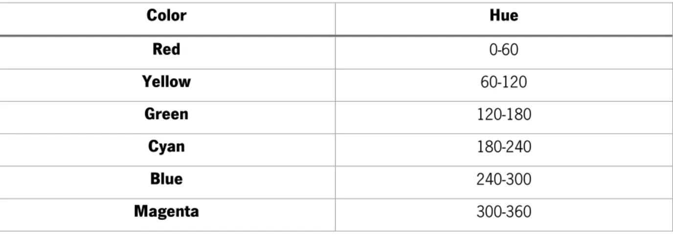
Figure 37 - Conversion of BGR to HSV. Where (a) is the source frame and (b) is the HSV frame ... 58

Figure 38 - BGR and HSV values of the clicked position ... 59

Figure 39 - Color Segmentation ... 60

Figure 40 - Result of the acquisition model using color segmentation ... 60

Figure 41 - Background (a) and foreground (b) frames ... 61

Figure 42 - Acquisition model with background subtractor ... 62

Figure 43 - Acquisition model with MOG background subtractor ... 63

Figure 44 - Segmentation with MOG background subtractor, where (a) is the background frame and the respective segmentation and (b) represents the frame with the object, foreground, and the correspondent segmentation. (a) and (b) are successive frames. ... 63

Figure 45 - MOG background subtractor segmentation, where (a) is the background frame and (b) is a consecutive frame and the respective segmentation. ... 64

Figure 46 - Acquisition with the arm ... 65

Figure 47 - Segmented frame ... 65

Figure 48 - Application of the bitwise NOT operation on the MOG mask (a) and on the color segmentation mask (b), resulting on the final mask (c) ... 66

Figure 49 - Final Acquisition framework ... 67

Figure 50 - Initial windows of the acquisition algorithm, where (a) is the main frame and (b) is the MOG mask. ... 67 Figure 51 – Color segmentation and MOG segmentation with the arm and the desired object. (a) is the

Figure 53 - Saved image frames and the respective files with the ground truth information ... 70

Figure 54 - Bad arm segmentation ... 71

Figure 55 - Bad MOG segmentation ... 71

Figure 56 - Training AP precision curve on Tensorboard ... 79

Figure 57 - Validation AP precision curve on Tensorboard ... 79

Figure 58 - Train the network ... 80

Figure 59 - Test frame with no NMS ... 81

Figure 60 - Test frame using NMS to suppress overlaps that are over 0.75 ... 82

Figure 61 - Test frame using NMS to suppress overlaps that are over 0.5 ... 82

Figure 62 - Test frame using NMS to suppress overlaps that are over 0.1 ... 83

Figure 63 - Frame rate ... 84

Figure 64 – Types of Bottles in the dataset ... 85

Figure 65 - Data1 training precision curves ... 86

Figure 66 - Data1 validation precision curves ... 87

Figure 67 - Data2 training precision curves ... 88

Figure 68 - Data2 validation precision curves ... 89

Figure 69 - Data2 training precision curves, with 150x150 as the input size... 90

Figure 70 - Data2 validation precision curves, with 150x150 as the input size ... 91

Figure 71 - Data2 validation precision curves, with different learning rates, with 20 epochs and 150x150 as the input size ... 92

Figure 72 - Data3 training precision curves ... 94

Figure 73 - Data3 validation precision curves ... 95

Figure 74 – Detection when the bottle is being grabbed ... 96

Figure 75- - Detection of various bottles in other perspective ... 96

Figure 76 – Bad bottle detection ... 97

Figure 77 – Types of cans in the dataset ... 98

Figure 78 - Training AP curves of the bottle class ... 99

Figure 79 - Training AP curves of the can class ... 99

Figure 80 - Validation AP curves of the bottle class ... 100

Figure 81 - Validation AP curves of the can class ... 100

Figure 82 – Training AP of Data 4 and Data5 curves of the bottle class ... 102

Figure 84 – Validation AP of Data4 and Data5 curves of the bottle class ... 103

Figure 85 – Validation AP of Data4 and Data5 curves of the can class ... 103

Figure 86 – Detections of a single object in a frame ... 104

Figure 87 – Detections of both classes ... 105

Figure 88 - Types of bag of chips in the dataset ... 105

Figure 89 – Training curves of each class ... 106

Figure 90 - Validation curves of each class ... 107

Figure 91 - Training curves of each class using 200x200 as the input size ... 108

Figure 92 - Validation curves of each class using 200x200 as the input size ... 109

Figure 93 - Bottle detections ... 110

Figure 94 - Can detections ... 110

Figure 95 - Bag of chips detections ... 111

Figure 96 – Network detections in more than one class ... 111

Figure 97 –Bad recognition ... 112

Figure 98 – Nonexistent detection ... 113

T

ABLE

I

NDEX

Table 1 - Precision and recall values ... 32

Table 2 - Comparison of results between Fast R-CNN and R-CNN (Data source [39]) ... 41

Table 3 - Timing (ms), for each image until it reaches the end of the network.(Data source: pag.8 [40]). ... 43

Table 4 - Difference on performance between two methods, both using Fast R-CNN object detector with VGG16 (Data Source: [40]) ... 44

Table 5 - Performance and speed of the object detectors, using the same dataset (Data source: [51]) 48 Table 6 - Results of the current leading object detection network using the same dataset (Data source: [53]) ... 48

Table 7 - Hue values and the respective color ... 59

Table 8 - Size of the SSD feature maps and the total number of anchors according to the preset size of the input layer ... 74

Table 9 – Input size of the feature maps ... 75

Table 10 - Results on Data1, with different number of epochs ... 86

Table 11 - Results on Data2, with different number of epochs ... 88

Table 12 - Results on Data2, with different number of epochs, with 150x150 as the input size ... 90

Table 13 - Results on Data2, with different learning rates, with 20 epochs and 150x150 as the input size ... 92

Table 14 – Results on Data3, with different number of epochs ... 94

Table 15 - Results on Data4, with different number of epochs ... 98

Table 16 – Final AP values of the network with 50 epochs, using the Data5 ... 101

Table 17 – Training AP values of the network using Data6 ... 106

Table 18 – Validation AP values of the network using Data6 ... 106

Table 19 - Training AP values of the network using Data6 and input of 200x200 ... 107

N

OMENCLATURE

API – Application Programming Interface ANN – Artificial Neural Network

AP – Average Precision

BGR – Blue Green Red

CNN – Convolutional Neural Network CPU – Central Processing Unit

DNN – Deep Neural Network

FN -- False Negatives FP – False Positives FPS – Frame Per Second FC – Fully Connected

GPU - Graphical Processing Unit

HOG – Histogram of Oriented Gradients HSV – Hue Saturation Value

ILSVRC – ImageNet Large Scale Video Recognition Competition IoU – Intersection over Union

mAP – mean Average Precision MOG – Mixture of Gaussian

NMS -- Non-Maximum Suppression

RGB – Red Green Blue

RCNN – Region Convolutional Neural Network RoI – Region of Interest

RPN – Region Proposal Network

SS – Selective Search SSD – Single Shot Detector SVM – Support Vector Machine

TN – True Negative TP – True Positive

1. I

NTRODUCTION

The visual information, even as Human beings, has a high relevance in the accomplishment of tasks as well as influences our behaviour in certain decision making. It is so important and complex that the Human brain has a part solely for visual processing, the visual cortex. It is where there is a vast amount of information that is obtainable and is why we strongly rely on our visual sense.

Therefore, artificial vision plays an important role in robotics since it has caused a great change in the paradigm of robotics, one of which is the capability of the robot to visually perceive the environment and interact with it to perform tasks such as, obstacle avoidance, object recognition and manipulation and Human interaction [1].

This dissertation is within the development of a service robot for domestic tasks with the goal of implementing a vision system that can detect objects presented in the environment to allow the robot their manipulation, and thus it addresses a computer vision problem on a robotic vision system.

According to [1], a computer vision problem aims for the understanding of a scenario, for example, detect objects, however, they are used for specific applications and for individual problems. On the other hand, a robotic vision problem treats the vision as one of the several sensory systems that the robot possesses which together are used to fulfil tasks.

Computer vision problems such as object classification, object detection and recognition and semantic segmentation requires a very deep understanding of image processing algorithms and thus they were very complex to implement due to image diversity and complexity as well as some factors that needed to be considered that increases the complexity of the vision problem, such as:

x The variations in viewpoint, that is, the same object can have different positions and angles in an image;

x The difference in illumination, where different images can have different light conditions; x The object could be partially hidden;

x The background clutter, that is, some objects might blend into the background.

Even with the introduction of machine learning algorithms, which brought rise to the development of systems that can learn from provided data, like the Human, according to Yann Lecun [2], the conventional machine learning techniques do not have the ability to process natural data in their raw form.

So, computer vision problems, before deep learning, were usually manually performed by applying a hand-crafted feature extractor to transform the raw data into a suitable relationship that,

afterwards, could be used by a learning subsystem (classifier) that could detect or classify the patterns in the input, for example “HOG” (Histogram of Oriented Gradients) features [3] and feature matching [4]–[6].

The deep learning has facilitated the resolution of these problems that previously required a high level of engineering. Indeed, deep learning methods can learn the representation of the raw input data and transform it successively to a more abstract representation to afterwards be detected or classified, and thus, according to [2], the key aspect of deep learning is that the features are learned from the data and not designed by Humans, and so they require “very little engineering by hand”.

1.1 General motivations

The deep learning systems, according to [7], has promoted a deep change in the pattern recognition, machine learning and computer vision communities since that most or all previous techniques are now based on deep learning methods. In fact, it has provided the possibility of implementing systems without “hard coding” them.

Yet, according to Yann Lecun [8], the conventional deep learning systems are unable to extract all the variants of computer vision problems, and so he devised a deep network for computer vision tasks named CNN (Convolutional Neural Network).

The CNNs have been in an uprising until nowadays, since that most computer and robotic vision problems now adopt this type of network as the main processing method, proving the added value of its use. Indeed, these networks have outperformed the previous deep learning algorithms in computer and robotic vision tasks, being that, with their constant evolution, they have also surpassed the Human in the accomplishment of classification tasks, like the ResNet architecture [9].

However, since these networks work with images, they have, in most architectures, millions of parameters, and therefore the usage of the CNNs require a high computation power, such as GPUs (Graphical Processing Unit), so most of the currently CNN based methods and architectures do not consider the usage of lower computation power such as CPUs (Computer Processing Units), which are way less expensive than the GPUs.

In addition, these networks, to precisely learn the properties of the data, need to be trained with a high quantity of images. Although there are online, datasets of images that are already prepared to

Moreover, these datasets not only remove the freedom of choosing the inputs and the outputs of the network, but also may have more outputs than necessary, or may not have the necessary outputs for the solution.

Thus, this dissertation will try to prove the viability of the usage of CNN even when using low end resources, such as CPUs, reinforcing the usage of CNNs in every machine vision problem. It will also prove that is possible to achieve good precision rates, even when using own made Datasets.

1.2 Objectives

The main goal of this dissertation is the development of an intelligent robotic vision system that can detect a set of objects presented in the environment in real-time and, therefore, it will be implemented a CNN-based vision system for object classification and detection using an own made dataset.

To achieve such goal the problem was divided by the following tasks:

x Study of the several CNN architectures developed as well as the state of the art CNN object detectors, to find the most suitable network to use in this solution;

x The development of the model framework, of which it will be divided in three main parts; i. The acquisition part, where the dataset will be created;

ii. The part where the network will be trained with the previously created dataset;

iii. The final part, named test, where the network, after being trained, is tested for the final application.

x The selection of the best dataset as well as the best parameters that represents the desired results, that is, the detection with a good precision rate in real time;

At last, after choosing the suitable dataset as well as the training parameters, it is intended to have a model that can detect the desired objects regardless of its position and perspective.

1.3 Structure of the Dissertation

According to the main objectives presented above, this dissertation is divided in four main parts. The first part or chapter 2, named literature review, is composed of the theoretical part of this dissertation in which, first, an introduction to the CNN is exhibited, where it is briefly presented why the conventional DNNs (Deep Neural Networks) were not appropriate to extract the feature on images. Afterwards, in the subsection 2.1 it is presented the main characteristics of a CNN which bought rise to this kind of

network. This will allow a better understanding behind the CNN and what are the differences in comparison the other neural networks.

Then, still on chapter 2, is shown the theoretical foundations, in subsection 2.2, where the concepts for this dissertation are demonstrated along with the chronological evolution of the CNN architectures and the respective performance. The subsection 2.3 is composed of the main state of the art object detectors networks developed as well as some applications on robotic vision problems in which it helps to verify which network is the best to use.

In chapter 3 the methods and methodologies used for the development of the prototype are demonstrated, since the acquisition of the dataset until the network testing. Firstly, it is revealed what are the materials (software and hardware) used for the development of the prototype. Afterwards, in subsection 3.1, the model framework is displayed to present the entire model, that is, the parts are briefly demonstrated and its supposed output. In the subsequent subsections (3.2, 3.3, 3.4), the parts are explained in detail along with the methods used to implemented them.

After the implementation of the model framework, the dataset and the parameters need to be tuned to choose the best combination that results on the best performance. Hence, the result chapter corresponding to chapter 4, is composed of the data and parameters selection of the model prototype displaying the results of each model with the different dataset and/or parameters along with the discussion of the results obtained.

In chapter 5 it is presented the conclusions of the realization of the prototype and of the obtained results, followed by the future work in chapter 6.

2. L

ITERATURE

R

EVIEW

The DNNs are an upgrade of the conventional neural networks, called ANN (Artificial Neural Network) that was first emerged as a learning algorithm in 1948 by Donald Hebb [10]. The main difference between the ANNs and the DNNs is the number of hidden layers in the network hence the name deep (figure 1).

Figure 1 – ANN and DNN standard architectures [11]

Each circle displayed in figure 1 is a neuron (the nuclear element of a neural network), also called node (figure 2). Each of them establishes a weighted connection with all the subsequent nodes [12]. The output value of any node is performed by an activation function or non-linearity, such as: The Sigmoid function; the Tanh activation; the ReLU (See also appendix A pag. 123).

Figure 2 – neural network node [13]

Yann lecun [8] refers that the traditional multi-layer network, as the DNN presented in figure 1 where all nodes in one layer are connected to all nodes on the next layer, are able to recognize raw images (usually size-normalized and centered) but they have some flaws.

For computers, an image is a multiple-dimension array of numbers and each number represents a pixel value, if it is intended to train an DNN to recognize something on images, then each input node should be a pixel. So, for example, if the dataset has a set of 30x30 images, then there should be 900 input nodes. If it is a colored image, i.e. an RGB (Red Green Blue) image the number of input nodes are increased by x3.

If the input is a high-resolution image the number of input nodes grows drastically. Hence, the number of totals parameters in a DNN grows sharply, increasing the computational resources needed to implement and train the network.

Still, the number of parameters may not stand a problem on some modern computers. According to Yann Lecun [8] the topology represented in figure 1 have no built-in invariance that uncovers the variations on the input images, namely, translations, scales and geometric distortions. Moreover, it completely ignores the strong 2D (Two Dimension) local correlation that images have, i.e. the pixels that are nearby are highly correlated.

2.1 Convolutional neural networks

The CNNs were introduced to uncover the drawbacks of the conventional DNNs being more robust and automatic in extracting features on images. The main characteristic of the CNN is that instead of connecting each neuron to all the previous ones, as in figure 1, it connects to a set of neurons located in a specific location in the previous layer, known as local receptive field [8] as shown in figure 3.

Figure 3 - Local receptive field [11]

neurons, on the test subject, that responds to different situations: the “simple cells” that are sensitive to orientations and the “complex cells” to movements, that is, to differences in positions. They concluded that the neurons in the visual system have local connectivity, hence the presence of local receptive fields, also the neurons on a layer perform the same kind of processing and the size of the receptive fields increases with depth [14], [15].

In conclusion, the CNN covers three architectural ideas which are, the local connections, the shared weights and spatial sub-sampling or pooling [8].

The local connections allow the extraction of features in an area of a feature map, i.e. they take advantage of the local correlation that the nearby pixels have, since they can form local features that are easily detected. On the other hand, Yann Lecun et al [2] states that the features of an image are invariant to location, that is, the feature can appear in any part of the image, hence, the idea of sharing weights in the same feature map allows the detection of the same pattern in any part of the image. Therefore, according to [2], the neurons or units in a convolutional layer are disposed in feature maps where each unit is the result of the local weighted connection of a set of units presented in the previous feature map. A set of units is the result of convolving a filter in a certain position of the previous map. The result of the convolution is passed through a non-linearity layer, usually the ReLu (see appendix A pag 123). All the units in the same feature map are the result of the application of the same filter in the previous map, hence they share the same set of weights. Nevertheless, different feature maps use different set of weights.

While the convolutional layer is responsible to detect the local features from the previous layers the pooling layer merges semantically similar features into one, by increasing the size of the receptive field. The convolutional layer and the pooling layer form the first stage of the CNN known as the feature extractor, while the last stage of the CNN is formed by the fully-connected layer [7].

2.1.1 Convolutional Layer

As the name says, the convolutional layer is a layer that performs convolutions on the input. The convolution is fulfilled by applying a filter or kernel that slides across the entire layer (figure 4).

Figure 4 - Applying a filter of 3x3x3 on the input layer

Each filter is composed by a set of weights, that are multiplied by the correspondent pixel values, during the convolving process, performing the product between the weights and the inputs. These filters learn, through training, to search for a specific feature in the input by “activating” when the feature is presented in the input layer [16].

In general, the convolutions at each location of the input layer can be represented as the weighted sum between the weights and the input values [17] as demonstrated in equation 1.

∗ + (1)

W represents the matrix of filter values, X the matrix of pixel values and b the bias factor.

The filter crosses all the layer, starting in the top left corner and ending at at the lower right corner, producing an output at every location. After applying the filter at each possible location, it results on an activation or a feature map, in this case a 18x18 map, as presented in figure 4.

The size of the output depends on a parameter that defines the number of steps that the filter moves, named stride (S), for example, the case presented in figure 5 the stride is 1, i.e. the filter moves 1 cell at each step. The representation in figure 5 demonstrates how the filter moves with the stride of 1 in a 10x10 map.

Figure 5 - Stride of 1

In figure 5, it is possible to see that the filter does 8 steps until it reaches the right end, and another 8 steps until the lower end, so the output map of that convolution is an 8x8 map.

The output size is defined by equation 2 [17],

− + 2

+ 1 (2)

where W represents the dimension of the input, F the filter size, S the stride and P is the amount of zero padding. The zero-padding consists on placing around the original map, a set of zero value pixels, as presented in figure 6. So, for W=10, F=3, S=1 and P=0, the output size will be 8.

The spatial size reduction that happens by performing convolution is not intended, because it will result in a sharp descent of the input volume, preventing deeper networks. Therefore, to prevent that size descent, it is usually used the zero-padding method as demonstrated in figure 6.

Therefore, by calculating the output size for P = 1, the output size will be 10, the same as the original map.

A typical convolutional layer is constituted by a stack of many activation maps, as the application of different filters results on various activation maps, that allows the extraction of multiple features at each location [8].

The depth of a convolutional layer is equal to the number of filters applied, for example if 5 filters were applied in the representation of figure 4, it would result in 5 activation maps, so the total volume would be 18x18x5.

In figure 7 is represented the features that each filter (boxes), is searching for a specific trained model, noting that the level of the feature increases in the subsequent layer.

Figure 7 - Visualization of activations in subsequent layers [18] 2.1.2 Pooling layer

By using the zero-padding method on the convolutional layer, the input size will remain the same as the input passes through the network, yet a size reduction is needed to carry out, as referred. The layer that does the reduction is called pooling or sub-sampling layer.

The size reduction is greatly needed for the feature extraction, because instead of just learning the exact relative positions between features, it allows the features to shift relatively to each other, making the network more robust to variations of the features (distortions, translations) [8]. Reducing the size allows to diminish the number of parameters, hence it gradually decreases the computational cost and complexity of the network.

The most common pooling methods are the max-pooling and the average pooling. The max pooling searches for the max value on the current filter position (figure 8) and the average pooling calculates the mean value (figure 9).

Figure 8 - Max-pooling, with filter size of 2x2, and stride 1

Figure 9 - Average pooling, with filter size of 2x2, and stride 1

2.1.3 Fully-connected layer

The fully-connected layer is performed once the spatial features are extracted, i.e. after the input image goes through a set of convolutional layers and pooling layers, hence it picks the high-level features and determines which features most correlate to a specific class [19]. It is the similarity that the CNNs have in relation to DNNs, where each pixel is considered as a separate neuron and each neuron is connected to all the previous ones [16].

The fully-connected layer extends all the output activation maps into a one-dimension vector, that is, the size of the first fully-connected layer depends on the size of the last map and the corresponding depth. The input vector is connected to a set of hidden layers following the output layer, that contains the output classes for the classification. An example of a fully-connected layer can be represented in figure 1.

A CNN is a combination of these layers, arranged in a specific way, and the number and the sequence of these layers depend on the way it was dimensioned [2].

Taking the example of AlexNet [20] presented in figure 11, the network is represented of 11 layers, excluding the input layer, and the corresponding sequence is:

x Conv->MaxPool->Conv->MaxPool->Conv->Conv->Conv->MaxPool->FC1->FC2->FC3(output layer).

The design of a typical CNN consists on defining the sequence and the structure of the layers. When the convolutional layers are defined it is necessary to select the number of filters that each layer will possess and the respective size as well as the intended non-linearity (see Apendix A pag 121). In addition, for the pooling layer, is necessary to choose the pooling operations, as well as the number of filters and their size.

2.2 Theoretical foundations

To implement a CNN model there are some factors that are needed to be considered as for example, if the network will train in respect to the ground truth, the nature of the output, the evaluation metrics to verify the performance of the network, the training processes, namely, the algorithms to train the network and the designing of the main architecture of the network. These concepts not only define the type of the network that will be used but also define the nature of learning process.

2.2.1 Supervised and unsupervised learning

Any machine learning application is divided into two groups based on the way they use the data to “learn”, the supervised and unsupervised learning. These methods define whether the data to train the network needs to be labeled or not.

The most common method is the supervised learning, where the network trains in respect to the ground truth, i.e. the network in the learning process expects not only the input image, but also the target label. Then, a supervised learning model needs the user to act as a guide to teach the model with the correct result and therefore it requires that the data used to train the network are labeled with the correct answers taking into account the outputs are previously known [21]. The supervised learning is usually used to train on classification and/or regression problems [22].

In opposition to the supervised learning there is the other method called unsupervised learning. This method does not need the output labels and the ground truth ones, because it infers the natural

2.2.2 Classification vs regression

Inside the supervised learning method there are two main algorithms which defines the nature of the output, known as the classification and the regression.

The classification problem is used when the desired output is a discrete label, more precisely, when the problem can be defined by a finite number of classes [23], for example, the MNIST dataset [24] is used to train a network to classify digits from 0 to 9 and therefore the output is composed of those 10 classes. Inside the classification problem there are two main types of classification, the binary classification and the multi-label classification [23].

The example presented above is a representation of a multi-label classification, where the model tries to detect what number is presented on the image from 0 to 9. The binary classification occurs when it is desired for the model to divide the predictions into two groups, for example, it is implemented a network to classify numbers, so the output should have only two labels, the numbers and the non-numbers (1 or 0), that is, it predicts if the supplied image contains a number, regardless of the number displayed.

On the other hand, the regression problem is used when the output is a continuous value, more precisely, when the output represents a quantity and not a set possible labels [23], for example, when it is intended to predict the price of a certain object.

2.2.3 Supervised Training

The training is the most important part of every neural network. It is where the network learns from data what are the corresponding features of a certain class, allowing them to properly predict the correct class in the input data. This learning process is performed by adjusting the network weights so that these values are the ones that best represent the model. In a CNN architecture the training will update the filter values to search for a certain feature in a class.

The supervised training process in a CNN is carried out the same way as DNNs, i.e. it is divided in 4 main tasks: the forward pass, the loss function, the backpropagation and the weight update [19]. The main goal of the training is to reduce the difference between the output predictions and the real output on a forward pass, by “discovering” the best suitable relationship between the input and the output [25]. The output prediction is the prediction of the network by the forward pass in the output layer. The real output is the information that is provided alongside the image, that is, the desired/target result.

The forward pass picks the image and passes it to the network and, at the end, a cost value is computed that indicates how bad the network is predicting the class, by calculating the loss function [26] which picks the actual predictions and the real output and calculates the error.

Afterwards, the backpropagation or the backward pass determines which values contributed most to the loss value computing the gradient of the loss function by propagating the error value through the network, from the output to the input, checking the contribution of each node to the output loss and therefore is checks how the change in the weights affects the loss, represented by the derivate of the loss function [25].

Once the derivate or the gradient of the loss is computed the weights are updated in a way that it minimizes the loss, that is, in an opposite direction of the gradient. The weight update is usually performed by an optimizer algorithm [27].

The set of the presented tasks (the forward pass, the loss function, the backpropagation and the weight update) represent an iteration or epoch. So, the training is performed for a fixed number of epochs, usually defined by the user. When all the epochs are executed, the model is trained [19].

For further understanding the neural network training procedure please see [28] and [17].

2.2.4 Intersection over Union

The IoU (Intersection over Union) is an evaluation metric, that is commonly used to measure how accurate a model is on predicting the position of an object, represented by its bounding box, in relation to the ground truth box.

To perform the IoU method, it is only needed the ground truth box, provided by the dataset, and the predicted box. The IoU (equation 3)[29], is a ratio that represents how much the predicted box is enclosed by the ground truth.

= (3)

The area of overlap or area of intersection, is the area that both boxes are overlapped, and the area of union is the whole area of both boxes (figure 10).

Figure 10 - Intersection and Union [30] 2.2.5 Average precision

The average precision (AP) value is the most common evaluation metric used to verify the performance of a neural network model by providing a precision value that “tells” how good a network is on performing a given task: if a network has a high average precision rate it can be implied that the network performs well the tasks otherwise the network behaves poorly.

The average precision is commonly calculated, per class, in every training epoch by using the 11-point interpolated average precision method [31]. This method consists in computing the precision and recall values to calculate the average of the maximum precisions at 11 recall levels.

The precision (equation 4) is the percentage of the predictions that are correct, that is, how accurate are the predictions.

On the other hand, the recall measures the amount of the truly relevant returned information and is represented by equation 5 [32]. = + (4) = + (5)

The method picks all the predictions provided by the network and sorts them according to their probability, from the highest to the lowest value, and verifies whether the predictions are positive or negative, by checking the IoU between the predictions and the ground truth, to after compute the

precision and recall values: if the IoU is less than 0.5 it means that the predictions are false, otherwise they are true.

If is considered that the entire dataset contains 3 images of a certain class, all the predictions of the network for that class are sorted as presented in table 1.

Table 1 - Precision and recall values

Rank Positive or Negative Precision Recall

1 True 1,0 0,3

2 Negative 0,5 0,3

3 Negative 0,3 0,3

4 True 0,5 0,7

5 True 0,6 1,0

For example, in the second rank the precision is = 0,5 and the recall is = 0,3.

According to the predictions shown in table 1, the precision and recall are related by the curve displayed in figure 11.

Figure 11 - Precision and recall graph

0 0,2 0,4 0,6 0,8 1 1,2 0 0,2 0,4 0,6 0,8 1 1,2 Precis ion Recall

Precision-Recall

Therefore, for each recall value, , from 0 to 1 in increments of 0.1, the precision is interpolated by replacing it with the highest precision in the next recalls ≥ [31] (equation 6) , resulting on the red curve represented in figure 12.

( ) = ( ) (6)

Figure 12 - precision interpolation

The average precision is then calculated by averaging the maximum precisions of the 11 recall values (0, 0.1, 0.2, … ,0.9,1), given by the equation 7 [32]. It also can be represented as the area under the red curve (figure 12).

= 1

11 ( )

∈{ . ,…, , }

(7)

So, in this example the AP is ( ∗ , ∗ , ) _{= 0,75.}

The mAP (mean Average Precision) is just the mean over all the average precisions obtained in every class. 0 0,2 0,4 0,6 0,8 1 1,2 0 0,2 0,4 0,6 0,8 1 1,2 Precis ion Recall

Precision-Recall

2.2.6 Convolutional neural network architectures

The convolutional neural networks are quiet a new feature that was introduced and propelled the field of deep learning. Even though the first convolutional neural network architecture was developed by Yann Lecun et al [8], in 1998, named LeNet-5, and can be presented in figure 13.

Figure 13 - Lenet 5 architecture [8]

The LeNet-5 architecture was fundamental to the field of deep learning for image recognition, since it was the first to state that image features are distributed across the image and the application of convolutions, more precisely, filters across the image, with learnable parameters was the best way to extract those image features [8].

As shown in figure 13, the network consists in several layers, such as:

x Input layer, is the beginning of the network, where the input raw image is provided; x Convolutional layer, is the result of the convolution applied at the previous matrix;

x Subsampling, reduces the spatial size, the result of subsampling consists on the Pooling layer; x Fully-connected-layer, puts the final set of matrices into a one-dimensional vector and allows

each neuron (pixel) to receive data from all the neurons in the previous layers; x Output layer, is where the classification is presented.

The sequence of this layers is a convolutional neural network, and these layers are the root of all the recent architectures of convolutional networks.

From 1998 to 2012 there was no further investigation in this area, due to computation incapacity to process these kinds of networks, at that time, because of the inexistence of GPUs and high-performance CPUs, and also due to the scarcity of image data.

Henceforth, the development of new architectures was possible with the evolution of computers, namely, faster CPUs and the introduction GPUs, and because of the constant increasing of image data in the internet.

Then, in 2012, it was introduced a new architecture of convolutional neural network, presented by A. Krizhevsky et al [20], named AlexNet. (figure 14) It is a network like the LeNet-5 architecture, presented above, but with more layers, that is, deeper.

This network was developed to classify over 1.2million high resolution images in the ILSVRC (ImageNet Large Scale Video Recognition Competition) 2012 contest [33]. The ILSVRC, is an image classification contest, where teams develop neural networks, to classify a set of images in 1000 classes. The AlexNet network achieved a top-51 error of 15.3% [34], a good result compared to the later years contestants,

that had an error rate above 25% [35].

Figure 14 - AlexNet architecture [20]

The introduction of this network revolutionized the area of deep learning, which proved that CNN can be used to learn complex features on images and that was the network that drove its constant development.

In the next year, in 2013, P. Sermanet et al. [36] presented a CNN architecture, named Overfeat,, which was in the ILSVRC–2013, with 29.8% of top-5 error on Classification plus localization challenge, and with 14.1% [37] on the classification competition. Even though, this network was a derivate from AlexNet, it obtained better results on the contest, demonstrating that if a CNN is trained not only to classify, but to detect and locate objects in images it boosts the network performance. The introduction of this network brought a novel method for localization and detection by accumulating predicted

bounding boxes, that later gave rise to other case studies, like the R-CNN architectures [38]–[40], which is the one of the current leading approaches for object detection.

Also, in the same year, many other new CNN were developed, for example the ZFNet [41], which was one of the best networks on the classification task, obtaining 13.5% [37] of top-5 error on the challenge. In 2014, there was developed two new architectures that had outstanding results on the ILSVRC-2014 contest, the GoogleNet [42] and the VGG network [43], with 6.6% and 7.3% [44] respectively, of classification top-5 error rate.

The VGG network proved that deeper networks can learn more complex patterns and thus have a better performance in image recognition. The VGG creators developed various architectures as displayed in figure 15, whose difference is the depth of them, that is, the number of layer that each network possesses.

Figure 15 - VGG configurations [43]

The main problem is that if the network is deeper, more parameters must be computed, and thus it is more computational expensive, so the VGG architecture has 3x3 filters on all the convolutional layers, to reduce the number of parameters to be calculated. It is still one of the most used network in the object detection architectures, since it has proved that can reach a good level of abstraction. However, in comparison to the GoogleNet it is somewhat computationally heavy.

and in the same time to maintain the performance of previous CNNs showing that CNN layers do not need to be stacked up sequentially.

Figure 16 - Inception Module [42]

At first glance, the Inception module is the combination of parallel convolutional filters (1x1, 3x3 and 5x5), that are applied to the input layer (Previous layer), and in the end, they are all concatenated. The GoogleNet network consists on a stack of Inception Modules.

The main insight of this Module is the usage of 1x1 convolutional filters after convolutions. The 1x1 convolutional filters were firstly used by M. Lin et al [45], that developed a neural network called network-in-network “NiN”. The NiN consists of a network with mainly 1x1 convolutional filters, that were used to provide more combinational power to the features of convolution layers. The usage of 1x1 convolutional filters allows the reduction of operations to compute, and thus it is less computational expensive.

The best architecture developed in the ILSVRC was the ResNet [9], in 2015, which won the contest with a 3.6% [46] error rate. Considering that Humans, in general, has an error rate between 5% and 10% the ResNet network outperformed the Human in classifications tasks.

Not only the network had excellent results on the classification contest but also established new records on the localization and detection tasks reaching an error of 9%.

The ResNet or deep residual network consists on a deep net with 152 layers of depth (much deeper than the previous year’s architectures) and introduced the idea of residual learning to deep neural networks. In this architecture, each layer of depth is called residual block (figure 17).

Figure 17 - Residual Block [9]

The residual block basically applies a set convolutional filters to the input x, and the result of those filters is added to the original input. The main difference of this feature on the previous architectures, is that, instead of computing the whole transformation of the input, that is, x to F(x), this residual block allows to only compute the variation of the input.

The vantage of the usage of this residual block is that makes the backpropagation process easier, because of the adding operation that distributes the gradients.

These architectures previously stated are the main developed CNN until nowadays, which express the evolution of this area of study over the years, and the importance of the ImageNet classification challenge on the evolution of CNNs. They are important to this case study, since most projects or applications, in this area, employ these architectures as the core of their algorithm, such as the object detection networks.

2.3 State of the art

Recently, due to the evolution of the CNNs presented above, there were developed some CNN-based models that had outstanding results in the object detection task. As presented above, the concept of predicting bounding boxes introduced on Overfeat network [47], gave rise to the development of CNNs whose purpose is the detection and recognition of objects with high performances and lower frame rates, named: RCNN (Region Convolutional Neural Network); SSD (Single Shot Multibox Detector); YOLO (You Only Look Once).

YOLO) performs the detections in a different way, handling the detections as a regression problem, called regression-based object detectors.

2.3.1 Region based Convolutional Neural networks (R-CNN)

The R-CNN, was one of the firsts networks that took advantage of the CNNs qualities to accurately detect objects on images.

The R-CNN, displayed on figure 18, presented by R. Girshick et al [38], in 2014, instead of using a sliding window method to generate the image patches to be fed to the network, it uses an algorithm called Selective Search (SS) [48]. The Selective Search reduces the number of boxes to be passed to the network, to around 2000, and by using local features like color, intensity, textures it generates all the possible location of the objects [38].

Figure 18 - R-CNN architecture [38]

Once the proposals are obtained, each region is modified to be a fixed size square and it is passed to a CNN, as shown in figure 18, it can be any of the CNNs stated above. Then at the end of the network, each region is classified, to predict if it is an object, and if so what object.

The final step, of this network is to find the box that perfectly fits the dimensions of the object, this is performed by running a linear regression algorithm on the region proposal.

In general, the R-CNN follows these 3 steps [38]:

1. Generation of the region proposals, by running Selective Search;

2. Each region proposal is cropped or warped, into a fixed size box, and fed to a pre-trained CNN, followed by a SVM classifier to get what is the object on that box;

3. Optimize the region proposals by the usage of a linear regression model, after it has been classified.

Even though, R-CNN was very slow, because all the 2000 region proposals obtained by the Selective Search had to be fed to the network, one by one with no shared computation, and in addition the whole training method involves running three separate models [39], which are: the CNN for image classification, on each proposal, the SVM classifier and the linear regression model. Therefore, it makes the train pipeline very complex, that is, slower to train.

With the goal of increasing the speed of R-CNN, it was introduced the concept of Spatial Pyramid Pooling (SPP) on SPPnets, in 2014, by K. He et al [49].

The SPP allowed to share the computation on the region proposal method, by firstly, computing a convolutional feature map for the entire input image, and thus generating the proposals on the last layer, by applying the SPP layer on top of it. Afterwards, each proposal is fed to a fully connected layer to be classified [49].

The SPP layer on figure 19 picks the region proposals obtained in the last CNN layer by any region proposal method, and for every region proposal it outputs multiple feature maps of different sizes (4x4, 2x2, 1x1), by using max pooling. Then, all the feature maps are concatenated into a fixed length vector, to be fed to a fully connected layer.

Figure 19 - SPP layer representation [49]

In general, the SPP eliminate the need of applying a region proposal generator in the raw input image, that is, it is not needed for each proposal to pass on the whole CNN, hence reducing the computational cost of running the CNN model various times. Also, it brought the possibility of passing to the network

However, like R-CNN, training a SPPnet also involves multi staging, that is, running models separately, the feature extractor, training SVMs and the regression model, that increases the training pipeline. To address the weaknesses of R-CNN and the SPPnet, it was, in 2015, implemented a new R-CNN network, named Fast R-CNN [39] exposed in figure 20.

Figure 20 - Fast R-CNN network [39]

The Fast R-CNN took advantage of the method used in the SPP to first obtain the CNN representation of the input image, and then applying the region proposals on that representation. But, instead of applying the SPP on the last layer, it is applied a pooling operation developed by the authors of Fast R-CNN, named RoI pooling. Afterwards, each proposal is classified, by a Softmax classifier, and in parallel the bounding box is optimized by using a linear regression [39].

The new contribution that this network brought is the usage of a new type of pooling, namely the RoI pooling, and the aggregation of the feature extractor, the classifier and the linear regression into one single model, rectifying the drawbacks of R-CNN and SSPnet and speeding up the training process [39]. The RoI pooling works similarly to the SPP, although instead of outputting multiple features maps, it only outputs one, whose size is defined previously.

This new network achieved outstanding results, in both training and testing speed (table 2), in comparison to the R-CNN architecture.

Table 2 - Comparison of results between Fast R-CNN and R-CNN (Data source [39])

R-CNN Fast R-CNN Speedup

Train time(h) 84 9.5 8.8x

Note that both the R-CNN and the Fast R-CNN have the VGG16 as the main CNN for the feature extraction, and the time consumed by the region proposal algorithm, in this case the Selective Search, is not included.

Even with all the enhancements in train and test times, as can be seen in table 2, the Fast R-CNN has a flaw, it still needs a separate algorithm to generate the region proposals. As the region proposal model is very expensive, the whole process could still be improved.

In view of that defect, Ren et al [40], in 2016, developed a new solution to speed up the Fast R-CNN model by integrating the region proposal model into the R-CNN model, they called it faster R-CNN (figure 21). The integration of the region proposal model, was achieved by implementing a Region Proposal Network (RPN) on the network.

Figure 21 - Faster R-CNN [40]

As stated above the region proposal methods, like Selective Search, search for local features on the image and draw boxes on the possible objects [48]. Then, the authors took advantage of the CNN feature extractor to run their region proposal solution.

The RPN consists on running a sliding window on the feature map and every window location is matched with a set of anchors, more precisely, with a set of boxes with different aspect ratios as represented in the figure 22 [40].

Figure 22 - RPN [40]

So, for each window location there are k possible region proposals, therefore, for each anchor is outputted a class score, that is, the probability of a class to be presented on the anchor, and the corresponding bounding box. The use of different aspect ratios allows the model to more accurately fit the box on the object, because the objects can have multiple shapes and aspect ratios [39].

Posteriorly, each bounding box obtained by the RPN, that most likely has an object, that is, with high probabilities, are passed to end part of the Fast R-CNN that classifies each box and by the regression model it adjusts the box on the object.

The faster R-CNN (figure 21) is represented by one single model, i.e. there is no need of performing outside processes, the network outputs all the possible object with their corresponding bounding box and score for each box.

This new architecture improved once more the speed of the network, because as stated on table 3 the region proposal network is almost cost free, in comparison to others region proposal algorithms.

Table 3 - Timing (ms), for each image until it reaches the end of the network.(Data source: pag.8 [40]).

Model System Conv Proposals

Region-wise2

Total Rate

VGG SS + Fast R-CNN 146 1510 174 1830 0.5 fps

VGG Faster R-CNN 141 10 47 198 5 fps

2 The region-wise is all the processes before the region proposals, namely, the RoI pooling, the fully-connected, the classifier

By analyzing the results that were obtained, by the authors, the faster R-CNN performed 10x faster than the Fast R-CNN. This enhancement happens mostly because of the RPN, as shown, it only takes 10ms to be performed. On the other hand, the SS takes 1510ms, that is, much slower.

The authors also proved that, the faster R-CNN not only perform the object detection in a faster way, but also it has better results in terms of precision, i.e. the precision of the network in detecting an object as represented on table 4.

Table 4 - Difference on performance between two methods, both using Fast R-CNN object detector with VGG16 (Data Source: [40])

Method #proposals Dataset mAP

SS + Fast R-CNN 2000 VOC2007 66.9

SS + Fast R-CNN 2000 VOC2007+VOC2012 70.0

Faster R-CNN 300 VOC2007 69.9

Faster R-CNN 300 VOC2007+VOC2012 73.2

Until the introduction of the R-CNN there was, as presented above, a chronological evolution of the original architecture with the goal of improving it, in terms of speed and precision, and as proved the faster R-CNN is the culmination of that evolution, having outstanding results in both time and precision. However, in 2017, it was introduced a new R-CNN architecture called Mask R-CNN [50], whose finality was to, along with faster R-CNN, perform image segmentation on each proposal. Establishing a new paradigm in R-CNN networks, that is, not just only locate the object with bounding boxes but it also locates the exact pixels of an object. The Mask R-CNN framework is represented in the figure 23.

The Mask R-CNN adds to the faster R-CNN a portion that performs the mask, as it shows on figure 23, that is, it predicts if a given pixel is part of an object or not. That portion is just a set of convolutional layers on top of the feature map.

Still, the authors had to make a change on the faster R-CNN model to improve it, namely, on the RoI pooling, because the RoIPool slightly misaligns the boxes from the regions on the original image. Hence, as the pixel-level segmentation requires a more accurate method, the authors developed the RoIAlign [50]. The whole network can be represented in figure 24.

Figure 24 - Mask R-CNN architecture [50]

When the masks are generated they are combined with the region-wise part of the faster R-CNN, namely, the classifications and the bounding boxes, as presented in last part of figure 24, to perform the segmentation and the classification on each object.

2.3.2 You Only Look Once (YOLO)

The YOLO model was introduced in early 2016, by J. Redmon et al [51] and achieved a frame rate of 21fps, much faster than the faster R-CNN.

The YOLO model achieved that results because it performs the whole process of detection with only one pass, that is, a single pass on the whole network predicts at the same time the bounding boxes and the respective class probabilities. In addition, instead of just “see” the region proposals, the YOLO “see” all the input image, therefore, it promotes a better distinction between the objects and the background, enhancing the precision of the network [51].

The YOLO system as shown in figure 25, divides each image into a grid of SxS squares, and each square is responsible to predict a set of bounding boxes and a confidence score for each box.

Figure 25 - YOLO model [24]

The confidence is a probability score where, in this model, it tells how accurate is the bounding box and the probability that a certain object is enclosed by that bounding box. It is defined by equation 8 [51].

Pr( ) ∗ (8)

Then, if the object exists on that cell, the confidence score should be the IoU between the predicted box and the ground truth [51].

Afterwards, each grid cell also predicts the class probabilities for each class, represented by the class probability map on figure 25.

Then the confidence score for each bounding box and the class prediction are combined into one final score as shown in equation 9 [51], that outputs the probability that a certain bounding box contains a specific type of object.

Pr( |Object) ∗ Pr(object) ∗ = Pr( ) ∗ (9)

The result of the class-specific confidence score is represented by the final detections, however, note that the final detections on figure 24 are thresholded, that is, it only shows the bounding boxes that have a confidence value above the threshold value.

Figure 26 - YOLO CNN architecture [51]

The architecture is composed of 24 convolutional layers (Convolutional and Pooling) followed by 2 FC layers, inspired by the GoogleNet architecture, but instead of using the inception model, they used 1x1 convolutional layer followed by a 3x3 conv layer in similarity to the network in network [51]. In the overall architecture, it is important to note that the last layer is a 7x7x30 matrix.

The 7x7 represents the divisions of the image, that is, the image was divided in 7x7 grids. The x30 represents all the values that each grid cell computes, more precisely, the bounding boxes and all the class probabilities. Hence, the last layer, computes the bounding boxes and the respective class for each cell.

The last layer of Yolo can be defined by equation 10 [51],

∗ ∗ ( ∗ 5 + ) (10)

Where S represented the size of each grid, B the number of bounding boxes for each cell and C is the number of classes.

The YOLO model achieved one the bests frame rates (45fps) of object detection networks, however, it has some limitations that can be relevant depending on the application. The major limitation is that the YOLO model struggles to detect objects that appears in a small group, because each grid cell can only have one class and have a limited number of bounding boxes to predict, defined by B, and it has difficulties to generalize objects that may have unusual aspect ratios or configurations [51].

Being that the YOLO, in comparison to the faster R-CNN, it is a model with less precision on detecting objects as proved in table 5.

Table 5 - Performance and speed of the object detectors, using the same dataset (Data source: [51]) mAP FPS Fast R-CNN [19] 70.0 0.5 Faster R-CNN VGG-16 [12] 73.2 7 Faster R-CNN ZF [12] 62.1 18 YOLO VGG-16 [24] 66.4 21

Besides the original YOLO model, there were developed new models that had better performance, namely, the YOLOv2 or YOLO9000 [52].

2.3.3 Single Shot Multibox Detector (SSD)

The SSD is also one of the main object detection networks, based on a regression problem and has outperformed both faster R-CNN and YOLO in both accuracy and speed tasks and is current the best object detection system that has the perfect balance between speed and accuracy.

The SSD (figure 27), was introduced in late 2016, by W. Liu et al [53], and has achieved an accuracy of 74%mAP at 46fps, the table 6 represents the results of SSD in comparison to the other leading object detectors.

Table 6 - Results of the current leading object detection network using the same dataset (Data source: [53])

Object detector mAP FPS #Boxes Input resolution

Faster R-CNN (VGG 16) 73.2 7 6000 1000x600

YOLO (VGG 16) 66.4 21 98 448x448

SSD300 74.3 46 8732 300x300

SSD512 76.8 19 24564 512x512

The table above proves that the SSD has relatively good results regarding both accuracy and frame rate, even with more detections, represented by the number of boxes.

F

Figure 27 - SSD architecture [53]

The SSD network is built on a standard VGG-16 architecture to extract the features maps, however, the fully connected layers are switched to convolution layers that progressively reduce the size of the input thus adding other feature maps at lower scales.

The main insight of the SSD model is that it performs the detections by applying a set of convolutional filters, of size 3x3, at each feature layer. The existence of multiple layers of different scales allows these predictions to be performed at multiple scales and ratios, contributing to a better performance. Each filter outputs a score for each class and a boundary box [53].

In addition, at each cell of a feature map, for multiple maps, is associated a set of default bounding boxes centered at that cell. Therefore, instead of predicting boundary boxes from a global coordination, the box predictions are relative to a default boundary box at each cell (figure 28).

Figure 28 - Multiple scale feature maps and default boundary boxes [53]

So, for each feature map cell it is predicted the box offsets relative to the default box with the correspondent class scores, that indicates the presence of a class.

In training the default boxes are matched to the ground truth ones, to determine which default boxes correspond to a ground truth. These matches are represented by positive and negative matches. The match is positive if the corresponding default box as an IoU over 0.5, otherwise it is negative [53]. This method of computing the matches, also known as Multibox [54], provides the starting point of the training, that is, instead of starting with prediction from a random coordinate, the predictions start with the positive matches and as the training progresses the predictions tries to fit the ground truth boxes [53]. For example, in figure 28 the ground truth of the cat matches the 2 two default boxes in the 8x8 feature layer, and the ground truth relative to the dog matches to one default box in the 4x4 feature layer, all the other boxes are considered negative matches.

Also, as shown in figure 28, each feature map is responsible to match a scale of the object. Then, for each feature layer is defined a scale for the default boxes that can be represented in equation 11 [53]:

= + −

− 1 ( − 1), [1, ] (11)

smin is the minimum scale, usually between 0,1 and 0.2, smax corresponds to the maximum scale, normally 0.9, and m is the number of feature layers.

Beyond the scale, it is also defined the different aspect ratios for the various default boxes, which usually are defined as follows, 1,2,3, , [53].

The size of the default boxes, width, in equation 12 [53], and height, in equation 13 [53], are calculated as follows:

ℎ = × (12)

ℎ ℎ = (13)

In addition, for the aspect ratio of 1 is defined an extra scale that is calculated by equation 14 [53].