J. Aerosp. Technol. Manag., São José dos Campos, Vol.7, No 3, pp.328-334, Jul.-Sep., 2017
ABSTRACT: In the present study relative state transition
matrix was obtained. It matches the relative motion of 2 satellites while including the oblate perturbation. The used formulation applies the geometric approach and is in Cartesian frame. The relative state transition matrix uses absolute state transition matrix of individual satellites. Thereon, simpliication in computing methods and on-board implementation at controls are explored in a leader/follower coordination method. Numerical experiments illustrate the accuracy when the baseline separation is equal to 2 km and eccentricity is 0.005 and 0.05 for all the inclinations.
KEYWORDS: State transition matrix, Formation lying, Orbit,
Oblate.
Relative State Transition Matrix Using
Geometric Approach for Onboard
Implementation
Mankali P Ramachandran1INTRODUCTION
Formation lying is about harnessing and controlling the relative orbital dynamics. When using multiple observations obtained from a formation of the low Earth orbiting satellites, the combined data is enhanced. he Clohessy-Wiltshire (CW) equation that describes a relative motion is valid for a small relative distance between the satellites compared to the radius and it assumes that the reference orbit is circular besides using a spherically uniform gravitational ield at the centre (Alfriend et al. 2010). In practice this is not true for a low Earth orbiting satellite. Maintaining a formation with respect to the circular reference orbit requires prohibitive fuel consumption. It needs frequent orbit corrections to reduce the deviations caused by perturbations. he irst signiicant perturbation is due to the
efect of oblate Earth denoted as J2. When the reference orbit is
initially nominally circular, a small eccentricity usually occurs due to the J2 efect, which also causes a regression in the orbital plane. It may be noted that an advanced scheduling of the satellite payload data collection on the Earth is usually based on a ground system. his mapping system uses an orbit model that includes mean oblate efect. hus, in general, it is more
important to include the J2 efect in the on-board reference
orbit of the satellite.
State transition matrix (STM) plays an important role in the orbit control. It occurs in the system dynamics equation that is used to control the satellite. he STM that is implemented on-board a satellite needs to be simpler, computationally efficient, and yet scaled close to match the accompanying reference on-board orbit model. Here, the reference orbit on
1.Indian Space Research Organisation – Satellite Centre – Flight Dynamics Group – Bangalore/Karnataka – India.
Author for correspondence: Mankali Padmanabha Ramachandran | Indian Space Research Organisation Satellite Centre – Flight Dynamics Group | Old Airport Road | 560017 – Bangalore/Karnataka – India | Email: [email protected]
J. Aerosp. Technol. Manag., São José dos Campos, Vol.7, No 3, pp.328-334, Jul.-Sep., 2017
329
Relative State Transition Matrix Using Geometric Approach for Onboard Implementation
each of the satellites is a irst-order motion that includes the J2
efect (Roy 1982). In this paper, it was obtained an approximate computationally simpler relative STM in Cartesian frame to match this relative motion.
here are various formulations of relative STM and each
assumes certain orbital characteristics (Alfriend et al. 2010).
Here a rectangular Cartesian frame is used since it helps in the direct use of GPS navigation systems data. Incrementing the maneuver velocity is easier to understand with respect to the orbit frame of reference. Cartesian frame has been found to perform satisfactorily under propagation for formation types that are not largely separated along-track (de Brujin et al. 2001).
he irst STM is that of the circular CW equation. he assumptions in the CW model, as mentioned earlier, are the limitations in its use. he STM is derived in Cartesian frame from the analytical solution of the CW diferential equation
(Alfriend et al. 2010). When the eccentricity of the reference
orbit is small, a STM can be derived in Cartesian frame, as carried out by Melton (2000). his involves a lengthy expression as a function of time and is a series with terms which are powers of
the eccentricity(Melton 2000). When the orbit is more elliptical
then the Keplerian one, it is transformed following the approach of Tschauner and Hempel (1965) to yield a closed form relative
motion. his STM given in Yamanaka and Ankersen(2002) is
an improvement made to Carter(1998). Here the independent
variable is the true anomaly. he time-explicit STM is easier to adopt in the control system.
he method of Gim and Alfriend (2003)has solved the
problem of STM, having matched the relative motion about
an elliptical orbit with J2 effect. Though the time-explicit
expression is analytical and accurate, it is laborious for on-board implementation. he model includes short and long periodic efects and is in terms of non-singular elements. It is important to mention that there is no need to include the long-period efects
under J2 perturbation. In Hamel and de Lafontaine (2007), this
is explored, and an alternative STM was presented, being valid for all cases when the reference orbit is not circular. It is based on mean orbit element diferences between 2 satellites. When the eccentricity is small, then a lesser complex version is given
in Alfriend and Yan (2005). he STM formulated in Yan et al.
(2004) is based on the unit-sphere method (Vadali 2002). he approximate STM in Tsuda (2011) is in Cartesian frame and involves a series for on-board implementation.
Here the approach is geometric, that is, it applies a geometric transformation between the relative states of the deputy with
respect to the chief and the orbital frame of the chief satellite. his was adopted to describe the relative motion in Balaji and Tatnall (2003) which is similar to the unit-sphere approach (Vadali 2002) and appeared at the same time. he relative motion described in
Vadali (2002)as well as in Balaji and Tatnall(2003) includes the
J2 efect, is applicable for eccentric orbits, and is valid for larger relative distances, using Keplerian elements. he present geometric approach is in Cartesian frame. he relative STM obtained here is approximate and explores optimized computation. Navigation plan suggested here is suited for on-board real-time usage
of STM in leader/follower coordination (Alfriend et al. 2010).
he STM is applicable for both osculating and mean elements of the 2 satellites. It also provides a scope of including secular efects due to higher-order perturbation. Finally, numerical experiments bring out the accuracy of state updated by the STM in terms of varying eccentricity and inclination.
REFERENCE ORBIT AND STATE
TRANSITION MATRIX
he orbital motion of the deputy and chief satellite with
J2efect is discussed next. he absolute STM of the 2 satellites
is then derived. his is required in each of the satellites in controlling their reference orbits.
he equation of motion of an individual satellite is (Roy 1982):
where R ¨ denotes the second derivative with respect to time
of R = (X,Y,Z).
he disturbing potentialis:
(1)
(2)
(3) with
where: μ is the Earth’s gravitational parameter, equal to
398,600.64 km3/s2; J
2 = 0.0010826; δ is the instantaneous
declination; Re is the Earth’s radius, which is 6,378.458 km;
R is the magnitude of the satellite position vector, R.
he position vector of the deputy and the chief satellites is denoted by Rdand Rc, respectively, in the Earth Centred Inertial
Frame (ECIF). he potential is axi-symmetric about the Z-axis
and is independent of the azimuth angle ψ.
F has 2 types of expressions (Roy 1982):
=∇U
ψ
δ
ω
/
/ /
/ /
/
ω / /
/ /
U(R,ψ,Z) = (/R) + F
δ
ω
/
/ /
/ /
/
ω / /
/ /
ψ
F = - (/R)(Re /R)2 J2 (1/2){ 3 sin2δ -1} ,
ω
/
/ /
/ /
/
ω / /
/ /
J. Aerosp. Technol. Manag., São José dos Campos, Vol.7, No 3, pp.328-334, Jul.-Sep., 2017
330 Ramachandran MP
for close formations to avoid any collision. On the other hand, having the reference to be a mean motion fuel is saved by having impulse maneuver used once or twice appropriately in the orbit
besides maximizing data collection duration (Gill et al. 2007).
Let Xj(t) = (Xj,Yj,Zj,X1
j,Y
1
j,Z
1
j) be in orbital state in the ECIF.
At the epoch (t0), the state is Xj(t0), where j = 1 denotes the state of the chief and j = 2 that of the follower.
he absolute STM formulation follows the method of Markley (1986). Equation 9 describes the potential and is in Cartesian frame when using periodic and secular terms:
(7) (9) (10) (11) (12) (4) (5.1) (5.2) where: F1 contains only the secular component while F2includes the short-period perturbation.
where f is the true anomaly.
he Lagrange’s planetary equation of motion (Roy 1982) is:
where:
where: a, e, and i are, respectively, the semi-major axis,
eccentricity, and inclination; ω, Ω, and M are, respectively,
argument of perigee, longitude of the ascending node and mean anomaly.
There are 2 kinds of reference orbits for on-board implementation on both satellites. It is either (a) osculating
and obtained by substituting F2 in Eq. 6 or (b) the mean
motion obtained by substituting F1 in Eq. 6. he latter is the
more familiar irst-order secular perturbation with a, e, and i
remaining constant, as it is at the start epoch. When mapping the orbit elements to the mean ones, only 3 orbit elements are
found to exhibit secular growth due to the J2 efect and are
where: Rj = (X2j + Y
j
2+ Z
j
2)1/2.
On the other hand, the potential for secular efects alone is:
he acceleration derived from the potential for the case (a) with secular and short periodic motion is presented as in Chairadia et al. (2012):
On the other hand, for (b), when only secular efects are considered, the accelerations can be seen in Ramachandran (2015) as:
where the constant α = −μRe 2J
2 (3/2) (1 − (3/2) sin 2(i)).
It can be noted that the inclination i is invariant in the
motion described in Eq. 8. These accelerations are then used to derive the partial derivative and obtain the absolute STM matching the 2 types of reference motions: (a) or (b). Details are given in Markley (1986), as well as in Chairadia et al. (2012).
RELATIVE STATE TRANSITION MATRIX
FORMULATIONNext, it is described the relative motion of 2 satellites by the geometric principle. he motion of the deputy satellite is
ψ
δ
F = F1 or F2
ω / / / / / /
ω / /
/ /
ψ
δ
F1 = (/R) (Re/R)2(J2/2) (1-(3/2)sin2(i))
ω
/
/ /
/ /
/
ω / /
/ / ψ δ
F2 = (/R) (Re/R)2 ( J2/2) [(1-(3/2)sin2(i))+((3/ ω
/
/ /
/ /
/
ω / /
/ / ψ δ ω
da/dt = (2/na) /
/ /
/ /
/
ω / /
/ / ψ δ ω /
de/dt = ((1-e2)/(na2e)) / - ((1-e2)1/2/(n a2e)) (/)
/ /
/
ω / /
/ / ψ δ ω / / /
di/dt = (cos(i)/(na2 (1-e2)1/2 sin (i))) (/) – (1/ /
/
ω / /
/ / ψ δ ω / / / / /
d/dt = (1/(na2 (1-e2)1/2 sin (i))) /
ω / /
/ / ψ δ ω / / / / / /
dω/dt = - (cos(i) /(na2 (1-e2)1/2 sin (i)) / + /
/ / ψ δ ω / / / / / /
ω / /
dM/dt = n – ((1-e2)1/2/( na2e)) / - (2/na) /
ψ δ ω / / / / / /
ω / /
/ /
n2a3 =
ψ δ ω / / / / / /
ω / + (1-e2)1/2/( na2e) /
/ / ψ δ ω / / /
/) – (1/(na2 (1-e2)1/2 )sin (i))) /
/
ω / /
/ / ψ δ
(i))+((3/2) sin2(i) cos(2(f+ω)) ]
/
/ /
/ /
/
ω / /
/ /
(6)
(8) ω = ωo + (3/2) J2 (Re /p)2ň {2 –(5/2)sin2 (i)} t
= 0 – (3/2) J2 (Re /p)2ň cos(i) t
ň = n0 [1 + (3/2) J2 (Re /p)2 [1-(3/2)sin2(i))(1-e2)1/2 ]
M= M0 + ňt
α α α
ω ω ň
ň
ň
ň
U = (/Rj ) – (/Rj ) (Re /Rj )2 J2 (1/2)((3Zj2/Rj2) -1)
α α α
ω ω ň
ň
ň
ň
U = (/Rj) –(/Rj)(Re /Rj)2 J2 (1/2) {(3/2) sin2(i) -1}
α
α
α
ω ω ň
ň
ň
ň
ax = -(Xj/Rj3) [ 1 + (3/2) (Re /Rj)2 J2 (1-(5Zj2/Rj2)]
α
α
α
ω ω ň
ň
ň
ň
ay = (Yj/Xj)ax
a = -(Z/R3) [ 1 + (3/2) (R/R )2 J (3-(5Z2/R2)].
α
α
α
ω ω ň
ň
ň
ň
az = -(Zj/Rj3) [ 1 + (3/2) (R/Rj)2 J2 (3-(5Zj2/Rj2)].
α
α
α
ω ω ň
ň
ň ň
ax = (αXj/Rj5) – Xj/Rj3
α
α
ω ω ň
ň
ň ň α
ay = (αYj/Rj5) – Yj /Rj3
α
ω ω ň
ň
ň ň α α
az = (αZj /Rj5) – Zj /Rj3
J. Aerosp. Technol. Manag., São José dos Campos, Vol.7, No 3, pp.328-334, Jul.-Sep., 2017
331
Relative State Transition Matrix Using Geometric Approach for Onboard Implementation
in the chief satellite’s local-vertical-local-horizontal coordinate
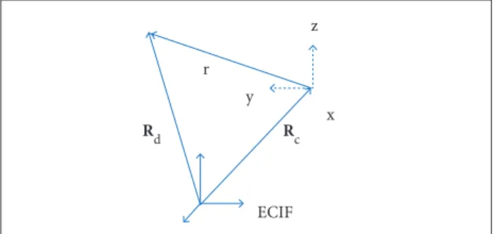
frame (LVLH). he relative position vector r, with respect to
the chief, has 3 components: x, y, and z, as illustrated in Fig. 1. Here, (x) is the component in the chief ’s radial direction, (z) is in the direction of the chief instantaneous angular momentum,
and (y) is along the direction that completes the triad (Alfriend
et al. 2010). he relative distance is:
where S = [RcRc1R
dRd
1]T.
Here [P] is a (6 × 12) matrix. In case the mean elements of
the state Š are used, then another transformation needs to be
carried out as in Gim and Alfriend(2003), in addition to that
of using Cartesian transformation.
(13.1)
(16)
(17)
(18)
(19.1)
(19.2)
(20) (14)
(15) (13.2)
he transformation matrix Coi (3 × 3) relates the LVLH frame
of the satellite to the ECIF. he position and velocity vectors are, respectively, Rc = (Xj,Yj,Zj) and Vc = (X1
j,Y
1
j,Z
1
j), where j = 1
denotes the chief satellite while Rd and Vd for j = 2 are used to denote the deputy satellite. he magnitudes are |Rc| and |Rd| for the chief and deputy satellites, respectively. he instantaneous angular momentum vector of the chief is Hc = (Rc × Vc), where
(x) is the usual vector cross-product. In Eq. (13.2), the second
row is the normalized cross-product of the irst and third rows. Taking the derivative of Eq. 13.1, the relative velocity is:
he transformation matrix D is reversible and has been
suiciently discussed by Gim and Alfriend (2003).
The following discussion uses osculating element. The formulation is analogous while using mean elements ater applying the transformation as in Eq. 16. he relative STM Φr(t,t0) follows:
with
The matrix P is known in Eq. 15. The second term
on the right-hand side of Eq. 18 is the matrix Q and it
uses the absolute STM derived earlier for both satellites.
If the input is the reference state S(t0), then the update is
obtained by using
Using Φa to individually denote the STM of the chief and
deputy satellites, we have
The matrices are the absolute STM obtained either (a) using periodic accelerations or (b) admitting only secular accelerations as mentioned in Eqs. 11 and 12, respectively. In case the relative STM for mean elements is needed, then the transformation for the osculating to mean, as in Eq. 18, is required.
In order to derive the elements of Coi 1 in P, a general relation is used
Figure 1. Relative motion of deputy satellite in the frame of the chief.
R
d Rc
r
z
y
x
ECIF
r = Coi [Rd – Rc ]
∆ Φ ∆ (17)
Φ
Rc / |Rc |
Coi = (Hcx Rc)/(|Hcx Rc|)
Hc/(|Hc|)
∆ Φ ∆ (17)
Φ
v = Coi [Rd 1
– Rc 1
] + Coi 1
[Rd – Rc ]
∆ Φ ∆ (17)
Φ
xrel = [P ] S
∆ Φ ∆ (17)
Φ
xrel = [ r,v]T
∆ Φ ∆ (17)
Φ
r = [ x,y,z] and v = [x1 ,y1 ,z1 ]
∆ Φ ∆ (17)
Φ
-Coi 0 Coi 0
[ P ] =
-Coi 1
-Coi Coi 1
Coi
∆ Φ ∆ (17)
Φ
Combining to get
S(t) = [ Q ] S(t0)
Φ
Φ
||
′
||
·′ ||
Φachief(t,t0) (6x6) 0 (6x6)
[ Q ] = (19. 0 (6x6) Φadeputy(t,t0)(6x6)
||
′
||
·′ ||
Φ
Φ
||
=
′
||
-
·′||
Substituting the 3 rows of Coi in place of (u/|u|) in the above
equation, it is obtained
S = D Š
∆ Φ ∆ (17)
Φ
∆xrel(t) = Φr(t,t0) ∆xrel(t0 ) (17)
Φ
∆ Φ ∆ (17)
J. Aerosp. Technol. Manag., São José dos Campos, Vol.7, No 3, pp.328-334, Jul.-Sep., 2017
332 Ramachandran MP
(21)
(24)
(25)
(22)
(23) Again the second row is computed as a cross product of the irst and third rows instead of the algebraic expression.
he matrix [T] in Eq. 18 is the inverse of matrix [P], and its new form is
he matrix multiplication can be further decomposed as: Φ
Φ
||
′ ||
·′ ||
Rc1/|Rc| - Rc(Rc.Rc 1T)/(|Rc|3)
Coi1 = [(Hc x Rc)1 /|(Hc x Rc )1 |] – [(HcxRc)((HcxRc).(HcxRc)1T )/(|HcxRc|3) (21)
Hc1/|Hc| - Hc(Hc.Hc1T)/(|Hc|3)
Φ
Φ
||
′
||
·′ ||
-Coi T
0
T = (1/2) -N -CoiT
CoiT 0
0 -CoiT
[α] = Coi(3x3)
β
γ Φ
δ Φ
α α γ α
β α β α λ α
Φ α
α
α
Φ α
α
α α
[β] = Coi 1
(3x3)
γ Φ
δ Φ
α α γ α
β α β α λ α
Φ α
α
α
Φ α
α
α α
β
[γ] = Φa chief
(t,t0) (6x6)
δ Φ
α α γ α
β α β α λ α
Φ α
α
α
Φ α
α
α
where: N = −Coi T C
oi
1T C
oi
T.
he relative STM Φr(t,
t
0) in Eq. 19 is approximate due totruncation in Q (Markley 1986).
COMPUTATIONAL REDUCTION
The computation reduction aspect is discussed next. The absolute STM are anyway needed on-board for individual orbit control. he additions for relative control are the matrices [P] and [T] and subsequently the matrix multiplication. It is now examined how this computation of the relative STM in Eq. 18 can be decomposed for computation eiciency. It may be noted that there are 4 matrices.
he relative STM Φr(t,t0) in Eq. 18 can be rewritten as
α
β
γ Φ
δ Φ
-α 0 α 0 γ 0 -αT 0
-β -α β α 0 λ N -αT
Φ ) = -αT 0
0 -αT
α
Φ α
α
α α
β
γ Φ
δ Φ
α α γ α
β α β α λ α
Φr(t,t0) = α
α
α
Φ α
α
α
γ Φ
δ Φ
α α γ α
β α β α λ α
Φ α
α
[ f ] αT [-f] 0
Φr(t,t0) = N αT
[-g ] αT [g] 0
0 αT
where: [f] = [−α 0 ] [γ] and [g] = [β α] [λ].
he repetition of matrices and 0 (3 × 3) matrices involved
in matrix multiplication helps to optimise the computation. he following navigation architecture further eases the computation.
he chief or target reference orbit is available in the deputy or follower satellite due to inter-satellite communication (Gill et al. 2007). he thruster on the deputy then controls the orbit to maintain the formation in a leader/follower coordination
(Alfriend et al. 2010). he chief reference orbit is undisturbed
during this operation. Using the states at t0 and t1, the elements of the matrix in Eq. 25 can be computed, ahead of that time. This management ensures that the elements of the first 3 rows of the matrix can be obtained beforehand. he orbit of the deputy or main satellite and the matrix [λ] alone varies due to orbit control thrusters and needs to be updated. his computational reduction in real time is the advantage of the present approach. On the other hand, in the case of unit-sphere approach (Vadali 2002), the transformation matrix in Eq. 15 is constructed using both chief and deputy states. Hence, all the elements of the relative STM need to be computed in real time and are task-intensive. he STM in Gim and Alfriend (2003) is more diicult for implementation.
J. Aerosp. Technol. Manag., São José dos Campos, Vol.7, No 3, pp.328-334, Jul.-Sep., 2017
333
Relative State Transition Matrix Using Geometric Approach for Onboard Implementation
Figure 2. Error variation with respect to inclination when e = 0.05.
!
Figure 2. Error variation with respect to inclination when e = 0.05.!
!
Position and velocity error, e = 0.05
Inclination [degree]
Inclination [degree]
P
os
it
io
n e
rr
o
r [m]
V
elo
ci
ty e
rr
o
r [m/s]
0.1
-0.1
-0.3
-0.4
0.1 0 -0.1
-0.3 -0.2
-0.4
0 30 60 90
0 30 60 90
Position and velocity error, e=0.005
Inclination [degree] Inclination [degree]
P
os
it
io
n e
rr
o
r [cm]
V
elo
ci
ty e
rr
o
r [cm/s]
1.5
-1.5 -3.0
-4.5 -6.0 0
0 30 60 90
0 30 60 90
1
-1
-3
-5
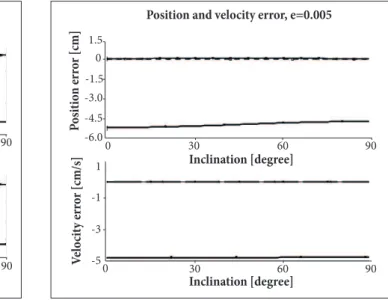
Figure 3. Error variation with respect to inclination when e = 0.005.
i s m o r e r e a l i s t i c t o a c c o u n t f o r s e c u l a r v a r i a t i o n w h i c h i s a l o n g t h e t r a c k b e t w e e n t h e s a t e l l i t e s i n f o r m a t i o n , a n d t h e S T M i s u s e f u l t o m a t c h t h e r e a l i s t i c m o t i o n o f t h e s a t e l l i t e.
NUMERICAL ANALYSIS
he experiment carried out here intended to estimate the
accuracy of the STM given in Eq. 17. The mean motion is selected as input for each equation. From Eq. 8, the initial states at times t0 and t1 are achieved, and the matrix [Q] is obtained.
Using the known relative position at time t1 as input and the
approximate STM in Eq. 17, the update of the relative state
at time t2 is obtained. This appears on the left-hand side of
Eq. 17. he time step selected is 1 s. Subsequently, it is obtained the diference between this output ∆xrel(t2) and the actual relative state at that instant computed using Eqs. 13 and 14. he error in position and velocity in the LVLH frame is related to the reference orbit. his error is gauged against variations in inclination and eccentricity. It is known that the J2 efect brings an out-of-plane (z) efect which is absent in CW equations. In the irst experiment, the orbital eccentricity is 0.05, and the semi-major axis a is 7,000 km. he deputy satellite is at a distance of 2 km along the track. he plot in Fig. 2 shows the error while varying inclination from 0 up to 90 degrees when retaining the eccentricity as 0.05. he numerical
accuracy of the methods from Gim and Alfriend (2003) and Yan et
al. (2004) shall be no diferent as they are mathematically similar
and difer in formulation. Also, the comparison of propagation error will be limited by the frame of reference. A case of higher
eccentricity when e = 0.1 is carried out. he error in the position and velocity was observed to be greater than that shown in Fig. 2, though the variation with inclination is similar. he errors in position and velocity are −0.68 m and −0.41 m/s, respectively. his increase in the error is as expected for higher values of e and
due to the approximation made in Q ofEq. 19.2.
It is seen that x and x1 (see Eqs. 13 and 14) have more perceivable error than (y, y1, z, z1). he position error is in the top plot while the velocity error is that at the bottom. he (y, z) values agree to 4 decimal places while (y1, z1) ones agree beyond 5 decimals. his implies that the update error along these axes is negligible.
To understand the efect of eccentricity, the experiment is repeated by changing the eccentricity to 0.005. he units now are in cm and cm/s — yet again the error is large in (x, x1). he error in the other axes agrees in 2 decimal places in position and 3 in velocity. When the distance of the satellites is 10 km, then the error gets proportionally scaled to that in Fig. 3. his is due to the approximation in the absolute STM.
he next test is carried out by varying the eccentricity from 0.0006 to 0.06. he inclination is ixed and equal to 20 degrees. In Fig. 4, the error along (x, x1) is greater again and increases
with eccentricity. It can be seen in Markley (1986) that the error in absolute STM depends upon the position in the non-circular orbit. In this example, the argument of perigee is retained while the eccentricity varies.
J. Aerosp. Technol. Manag., São José dos Campos, Vol.7, No 3, pp.328-334, Jul.-Sep., 2017
Figure 4. Error variation with respect to eccentricity when inclination is 20 degrees.
Variation in position error with eccentricity, inclination = 20o
Variation in velocity error
Eccentricity
P
os
it
io
n e
rr
o
r [m]
V
elo
ci
ty e
rr
o
r [m/s]
0.1
-0.1 -0.2
-0.3 -0.4 0
0 0.01 0.02 0.03 0.04 0.05 0.06
0 0.01 0.02 0.03 0.04 0.05 0.06
0
-0.1
-0.2
REFERENCES
Alfriend KT, Vadali SR, Gurfil P, How JP, Breger LS (2010) Spacecraft formation flying. Oxford: Butterworth-Heinemann.
Alfriend KT, Yan H (2005) Evaluation and comparison of relative motion theories. J Guid Contr Dynam 28(2):254-261. doi: 10.2514/1.6691
Balaji SK, Tatnall A (2003) System design issues of formation-flying spacecraft. Proceedings of IEEE Aerospace Conference; Big Sky, USA.
Carter TE (1998) State transition matrices for terminal rendezvous studies: brief survey and new example. J Guid Contr Dynam 21(1):148-155. doi: 10.2514/2.4211
Chairadia APM, Kuga HK, Prado AFBA (2012) Comparison between two methods to calculate the transition matrix of orbital motion. Mathematical of Problems in Engineering 2012(2012):Article ID 768973. doi: 10.1155/2012/768973
De Brujin F, Gill E, How J (2001) Comparative analysis of Cartesian and curvilinear Clohessy-Wiltshire equations. Journal of Aerospace Engineering, Sciences and Applications 3(2):1-15.
Gill E, Montenbruck O, D’Amico S (2007) Autonomous formation flying for PRISMA Mission. J Spacecraft Rockets 44(3):671-681. doi: 10.2514/1.23015
Gim DW, Alfriend KT (2003) State transition matrix of relative motion for perturbed noncircular reference orbit. J Guid Contr Dynam 26(6):956-971. doi: 10.2514/2.6924
Hamel J, de Lafontaine J (2007) Linearised dynamics of formation flying spacecraft on a J2 – perturbed elliprical orbit. J Guid Contr Dynam 30(6):1649-1658. doi: 10.2514/1.29438
Markley FL (1986) Approximate Cartesian state transition matrix. J Astronaut Sci 34(2):161-169.
Melton RG (2000) Time-explicit representation of relative motion between elliptical orbits. J Guid Contr Dynam 23(4):604-610. doi: 10.2514/2.4605
Ramachandran MP (2015) Approximate state transition matrix and secular orbit model. International Journal of Aerospace Engineering 2015(2015):Article ID 475742. doi: 10.1155/2015/475742
Roy AE (1982) Orbital motion. Bristol: Adam Hilger Ltd.
Tschauner J, Hempel P (1965) Rendezvous with a targets in an elliptical orbit.Astronautica Acta 11(2):104-109.
Tsuda Y (2011) State transition matrix approximation with geometry preservation for general perturbed orbits. Acta Astronautica 68(7-8):1051-1061. doi: 10.1016/j. actaastro.2010.09.016
Vadali SR (2002) An analytical solution for relative motion of satellites. Proceedings of the 5th dynamics and control of systems and structures in space conference; Cranfield, UK.
Yamanaka K, Ankersen F (2002) New state transition matrix for relative motion on an arbitrary elliptical orbit. J Guid Contr Dynam 25(1):60-66. doi: 10.2514/2.4875
Yan H, Sengupta P, Vadali SR, Alfriend KT (2004) Development of a state transition matrix for relative motion using the Unit-Sphere Approach. Proceedings of the AAS/AIAA Space Flight Mechanics Conference; Maui, USA.
CONCLUSION
Based on the geometric approach, a relative STM was