J. Aerosp. Technol. Manag. vol.9 número4 jatm v9i4820

J. Aerosp. Technol. Manag., São José dos Campos, Vol.9, No _{4, pp.503-509, Oct.-Dec., 2017}

ABSTRACT: Aiming to mitigate the aerodynamic heating during hypersonic re-entry, the aerothermodynamic optimization of aerospace plane airfoil leading edge is conducted. Lift-to-drag ratio at landing condition is taken as a constraint to ensure the landing aerodynamic performance. First, airfoil proile is parametrically described to be more advantageous during the optimization process, and the Hicks-Henne type function is improved considering its application on the airfoil leading edge. Computational Fluid Dynamics models at hypersonic as well as landing conditions are then established and discussed. Design of Experiment technique is utilized to establish the surrogate model. Afterwards, the previously mentioned surrogate model is employed in combination with the Multi-Island Genetic Algorithm to perform the optimization procedure. NACA 0012 is taken as the baseline airfoil for case study. The results show that the peak heat lux of the optimal airfoil during hypersonic light is reduced by 7.61% at the stagnation point, while the lift-to-drag remains almost unchanged under landing condition.

KEYWORDS: Airfoil optimization, Aerodynamic heating, Hicks-Henne type function, Airfoil parameterization, Surrogate model.

Aerothermodynamic Optimization of

Aerospace Plane Airfoil Leading Edge

INTRODUCTION

Aerospace planes (ASP) encounter severe aerodynamic heating during the hypersonic phase of atmospheric re-entry. Its reusable nature dictates that it should be able to shield the underlying structure from excessive temperatures during hypersonic light and still have good aerodynamic performance at the landing speed. Regarding the Space Shuttle, a double-delta wing coniguration was adopted to optimize the hypersonic light as well as to obtain a good lit-to-drag ratio for landing (Launius and Jenkins 2012).

Since Computational Fluid Dynamics (CFD) plays a critical role in the aerospace industry, airfoil optimization has been widely studied during the design process of a winged vehicle. Buckley and Zingg (2013) developed a weighted-integral objective function to perform multipoint aerodynamic shape optimization in which a range of operating conditions were involved. A 2-step approach was introduced to conduct the aerodynamic and structural optimization of the adaptive wing leading edge (Sun et al. 2013). Various algorithms were employed for the aerodynamic optimization. A novel global optimization algorithm based on the particle swarm one was developed and applied to a low-velocity airfoil optimization (Yang et al. 2015). Koziel and Leifsson (2014) proposed an approach utilizing the multi-objective evolutionary algorithm together with surrogate model to obtain the Pareto front of a transonic airfoil. Li et al. (2012) developed an eicient method using the response surface model and genetic algorithm to optimize the transonic airfoil. Xia and Chen (2015) performed the aerothermodynamic optimization of a hypersonic wing profile to decrease the maximum heat flux. However, research on the hypersonic

1.Nanjing University of Aeronautics and Astronautics – College of Aerospace Engineering – Minister Key Discipline Laboratory of Advanced Design Technology of Aircraft – Nanjing/Jiangsu – China.

J. Aerosp. Technol. Manag., São José dos Campos, Vol.9, No _{4, pp.503-509, Oct.-Dec., 2017} 504 Zhou C, Wang Z, Zhi J, Kretov A

aerothermodynamic optimization for ASP considering the landing aerodynamic performance, is still limited.

In this study, based on the Space Shuttle re-entry case, the aerothermodynamic optimization of an airfoil leading edge was carried out to alleviate the severe aerodynamic heating during hypersonic re-entry, while aerodynamic characteristics under landing condition were simultaneously considered. First, linear superposition method of analytic function with a modii ed Hicks-Henne type function was used for parametric modelling. CFD models for both hypersonic and landing conditions are described here. h en, the adopted optimization approach is presented, followed by a discussion on the optimized results.

SPACE SHUTTLE RE-ENTRY

DESCRIPTION

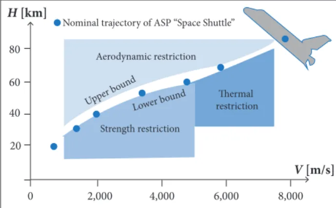
h e atmospheric re-entry is particularly challenging, and the Space Shuttle is designed for a predei ned schedule to survive the extreme environment (Launius and Jenkins 2012; Powers 1986). Figure 1 illustrates the nominal re-entry l ight corridor for Space Shuttle (Sellers 2004). It was controlled to l y at a 40° angle of attack, producing high drag, not only to slow it down to landing speed, but also to reduce re-entry heating. h e large amount of potential and kinetic energy is dissipated as heat as the Space Shuttle enters the atmosphere. A large detached bow shock wave carries away most of the heat, with the rest transferred to the vehicle through convection and radiation (Allen and Eggers Jr 1958; Tetzman 2010).

h e aerodynamic heating is the severest at the stagnation point. It is assumed that the stagnation zone was in chemical equilibrium. Although the gas behind the shock is most likely in a non-equilibrium state, the approximation of chemical

equilibrium boundary layer is reasonable in the stagnation zone. h e heat l ux at the stagnation point, which is the maximum heat l ux of the leading-edge, can be estimated by (Bian and Zhong 1986):

0 2,000

80

60

40

20

4,000 6,000 8,000

V [m/s]

H [km]

Nominal trajectory of ASP “Space Shuttle”

Aerodynamic restriction

Strength restriction

Thermal restriction Lower bound

Upper b ound

Figure 1. Re -entry corridor for Space Shuttle.

where: c and m are constants; ρ refers to the local air density;

ρ₀ is the air density at sea level; R_s represents the radius of curvature at the stagnation point; V is the vehicle’s velocity;

V₀= 7.9 km/s is the i rst cosmic velocity.

h e peak temperature of the outer surface is always close to the radiation equilibrium temperature. h e heat l ux arising from the aerodynamic braking should not cause the temperature on the ASP surface (T_w) to exceed the maximum permissible values for materials placed on the outer surface. As for the stagnation point,

where: σ = 5.67 × 10−8 _W/(m2_K4_{) stands for Stefan-Boltzmann} constant; ε is the emissivity of the surface, depending on the material processing and surface temperature.

At er a series of steep S-shaped banking turns, the vehicle lowered its nose into a shallow dive and began its approach to the landing site. h en the nose was pulled up to i nally slow down the vehicle to approximately 100 m/s at touch-down. Unlike commercial airliners, the Space Shuttle glides to runway with no power and has relative low lit -to-drag ratio, so it needs a big angle of attack to maintain the longitudinal l ying quality (Powers 1986).

AIRFOIL PARAMETERIZATION

h e airfoil proi le is regenerated through altering the value of the control points during the optimal design of 2-D airfoil, while parametric description tends to be more advantageous. h is paper uses the linear superposition method of analytic function to i t the airfoil proi le, which is dei ned from the baseline one, type function and corresponding coei cients, as:

(1)

(2)

(3)

1/ 2

0 0

( ) ( ) , m ws

s

c V

q

V R

ρ

ρ

≈

σε

∑

π

−



₋

₋







α

_π





≥

_

ρ

ρ

≈

4

,

w ws

T

q

σε

=

∑

π

−



−

−







α

_π





≥

_

ρ

ρ

≈

σε

1

,

n

b k k

k

y y a f

=

=

∑

π

−



₋

₋







α

_π

J. Aerosp. Technol. Manag., São José dos Campos, Vol.9, No _{4, pp.503-509, Oct.-Dec., 2017} where: – y_b (– x) represents the baseline airfoil proile; n and a_k are

the number of control points and the coeicients, respectively;

f_k (– x)denotes the type function; a_k f_k (– x) is the perturbation of the baseline airfoil.

In this paper, NACA 0012 is chosen as the baseline airfoil, which is similar to the airfoil for Space Shuttle Orbiter Columbia NACA 0012-64 (Rochelle et al. 1973). These airfoils have

the same leading-edge radius, and the only diference is the location of the maximum thickness. NACA 0012 airfoil can be described as:

NUMERICAL MODEL

COMPUTATIONAL FLUID DYNAMICS MODEL DESCRIPTION

he low around an airfoil is numerically simulated by solving compressible 2-D Navier-Stokes equations. he airfoil chord length is set as 5 m. C-type structured grids around the airfoil are generated by using the commercial sotware CFD-GEOM. Grid convergence studies are conducted, and approximately 4 × 105 _{cells are distributed in the domain. A close view of the}

mesh distribution is illustrated in Fig. 3. hen, the commercially available CFD-FASTRAN is employed to calculate both the heat lux at the hypersonic condition and the aerodynamic coeicients at the landing condition.

As for the hypersonic case in this paper, laminar low model is adopted since the air is thin and the Reynolds number is small at that altitude. Radiative wall boundary condition is used while the emissivity of the airfoil wall is assumed to be 0.8. It allows for radiation heat lux at the wall according to the Stefan-Boltzmann Law (see Eq. 2). hus, a balance is formed for heat lux at the wall between conduction to the wall and radiation from it. Regarding the landing condition, k-εturbulent model

with wall function is used to solve the problem. Since only the leading-edge is considered in this study, a

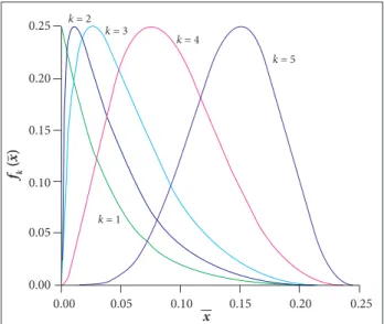
modiied Hicks-Henne type function (Hicks and Henne 1978; Zhou et al. 2014) is employed to control the irst quarter of the

airfoil proile, which is expressed as:

where: e(k) = 1n 0.5 / 1n x_k, 0 ≤ x_k ≤ 1, x_k= 4– x, x_k (k = 2, 3, 4, 5).

In this paper, coeicients a₁ ~ a₅and a₆ ~ a₁₀ are used to

control the upper and lower surfaces of the airfoil, respectively;

x_k (k = 2, 3, 4, 5) are set to be [0.04, 0.1, 0.3, 0.6]. he constraint a₁ = a₆ is applied to maintain the continuity of the airfoil leading

edge. he previously mentioned modiied type function with parameters setting is illustrated in Fig. 2.

Figure 2. Improved Hicks-Henne type function. 0.25

0.25

k = 1

k = 5 k = 4

k = 3 k = 2

0.20

0.20 0.15

0.15 0.10

0.10 0.05

0.05 0.00

0.00

x fk

(

x

)

Figure 3. Close view of mesh around the airfoil.

NUMERICAL MODEL VALIDATION Hypersonic Condition

According to a typical re-entry trajectory of Space Shuttle (Sellers 2004), its altitude and velocity proile is shown in Fig. 4. A series of hypersonic low simulations were conducted from 7,300 to 3,050 m/s through the re-entry stage, where the angle of attack was maintained at 40°. he heat lux variation with velocity at the stagnation point is shown in Fig. 5. Normally, the velocity for the maximum heat flux is about 80 – 85% of the re-entry velocity (Bian and Zhong 1986; Sellers 2004). In this study, the irst cosmic velocity is taken as the re-entry velocity. As shown in Fig. 5, the maximum heat lux occurs when the velocity decreases to approximately 6,700 m/s, i.e., (4)

(5)

ρ

ρ

≈

σε

∑

0 5 20

1

3

)

0

25

)

4 )

,

)

5sin [

4 )

], 1,

x

e k k

f x

x

x e

f x

π

x

k

−



=

−

−





=

>



α

_π





≥

_

506 Zhou C, Wang Z, Zhi J, Kretov A

roughly 84.8% of the re-entry velocity. hus, the CFD model used to calculate the heating results at the stagnation point under hypersonic condition is considered to be viable.

data (Ladson 1988) for NACA 0012 at high Reynolds numbers show that the airfoil will normally stall around α = 16°, which is

consistent with the numerical results obtained. he comparisons indicate that the numerical model is suitable for the landing condition problem.

Figure 6. Lift coeficient variation with angle of attack.

Figure 4. Space Shuttle’s altitude versus velocity for a typical re-entry.

80

70 60

50 40 30

20 10

0

0 2,000 4,000

V [m/s]

6,000 8,000

H

[k

m]

Flight data in reference Fitted curve

0

1.6

1.4

1.2

1.0

0.8

0.6

0.4

0.2

0.0

2 4 6 8 10 12 14 16 18

a[°] Cl

5.0

4.5

4.0

3.5

3.0

2.5

2.0

3,000 4,000 5,000

V [m/s]

6,000 8,000

q

[W/m

2]

7,000 × 105

CFD data Fitted curve

Start

Design

variables

Add samples

Design

of experiment

Response surface surrogate model

Accuracy evaluation

Multi-island genetic algorithm

Airfoil parameterization (MATLAB)

Meshing

(CFD-GEOM )

A e r o d y n amic analysis

(C F D - FASTRAN)

Exit

Landing Condition

Simulations of aerodynamic characteristics of the NACA 0012 airfoil were carried out at Re = 3.4 × 107 using the

previously described computational model. Angles of attack

α ranging from 0° to 16° were considered. Figure 6 shows the

lit coeicient variation with angle of attack. he slope of the lit curve for an airfoil at high Re can be estimated by the empirical

formula (Lu 2009):

Figure 5. Heat lux at stagnation versus velocity.

where: – c stands for relative thickness of the airfoil.

According to Fig. 6 and Eq. 6, the relative error of the lit curve slope between the CFD results and the empirical formula result is calculated to be less than 2%. he numerical result is very close to the theoretical one. In addition, experimental

OPTIMIZATION DESIGN

OPTIMIZATION APPROACH

he whole optimization process is shown in Fig. 7. All parts were integrated using the Isight framework (Dassault Systèmes Simulia Corp. 2012). Latin Hypercube Sampling (LHS; McKay

Figure 7. Designing process of optimization.

(6)

C

J. Aerosp. Technol. Manag., São José dos Campos, Vol.9, No _{4, pp.503-509, Oct.-Dec., 2017} 507 Aerothermodynamic Optimization of Aerospace Plane Airfoil Leading Edge

Flight condition

Altitude (km)

Pressure (Pa)

Temperature (K)

Velocity (m/s)

α

(°)

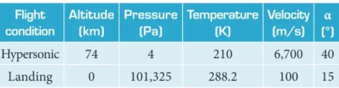
Hypersonic 7 4 4 2 1 0 6 ,7 0 0 4 0

Landing 0 1 0 1 ,3 2 5 2 8 8 .2 1 0 0 1 5

Table 1. Flight conditions used for optimization.

et al. 1979) was adopted for the design of experiment (DOE). Variables are normally referred to as factors in a DOE study, while the values are known as levels. With the LHS technique, the design space for each factor is uniformly divided, and then these levels are randomly combined to specify sample points defining the design matrix. It provides an efficient method for generating random sample points, which are uniformly distributed over the entire design space. For each sample, MATLAB® was used to automatically generate the corresponding airfoil proile database. hen, CFD-GEOM and CFD-FASTRAN were employed for meshing and low ield calculation, respectively; hypersonic heating environment, as well as landing performance, were also obtained.

Afterwards, surrogate models (Liem et al. 2015) are

established based on DOE results. Speciically in this study, Response Surface Method (RSM; Park et al. 2009) surrogate

models were used. he RSM is a statistical technique to explore the relation between design variables and responses. Low-order polynomials are usually applied to approximate the response of an actual analysis. A number of simulations, accomplished at the previous DOE stage, are required initially to construct a model. hen it can be used in optimization with a small computational cost, as only polynomial calculation is involved. For the current optimization problem, quadratic polynomial functions were adopted. Another set of random points in the design space were chosen to check these models. Surrogate models were continuously updated with additional sample points until the accuracy requirement was satisied. hen, these RSM models were used to replace the numerical ones in the following optimization process.

During optimization, the Multi-Island Genetic Algorithm (MIGA; Wang et al. 2015) was employed. Genetic algorithms (GA) are widely used due to their advantage to treat complex non-linear optimizations. MIGA, a further development of GA, divides each population of individuals into several sub-populations called islands, and traditional genetic operations are performed on each island separately. Several individuals are then selected from each island and migrated to diferent ones periodically. he migration operation maintains the diversity of probable solutions and prevents the premature phenomena.

OPTIMIZATION RESULTS

During this optimization study, peak heat flux at the stagnation point under the hypersonic condition was regarded as the objective function, while the lit-to-drag ratio at landing

condition was treated as the constraint. Coeicients of control points in Eq. 3 were taken as design variables. he optimization problem is described as:

where: K and K₀ refer to the lit-to-drag ratio of the optimal

and baseline airfoil, respectively.

According to the description in the sections “Space Shuttle Re-Entry Description” and “Numerical Model”, 2 typical light conditions were considered (Table 1).

Isight was used to integrate MATLAB® code, CFD-GEOM as well as CFD-FASTRAN to conduct DOE and the optimization process. First, 150 sample points were selected using LHS to conduct CFD analyses for both hypersonic and landing conditions, and the design space is: a₁, a₅, a₆, a₁₀ are among

[−0.01, 0.01], while a₂ ~ a₄ and a₇ ~ a₉ are among [−0.02, 0.02].

hen, RSM surrogate models were constructed for both objective and constraint functions. Another 20 random points were used to evaluate the accuracy of the surrogate model. Details are shown in Table 2, where RMSE stands for root mean square error. It is shown that the approximations for heat lux and lit-to-drag ratio are of high quality.

Table 2. Evaluation of the surrogate model.

Parameter RMSE

q_w 0.03587

K 0.03534

Aterwards, the surrogate model was used to replace the previous CFD models to carry out the optimization process. he critical parameters of MIGA are: the sub-population size is 10, the number of islands is 10, the number of generations is 30, the rate of crossover and mutation are 0.9 and 0.01, respectively, the rate of migration is 0.1, and the migration interval is 5.

he optimal results are shown in Table 3, where C_d represents

the drag coeicient. he characteristics of both baseline and

(7)

σε

∑

π

−



₋

₋







α

_π

0

,





≥

_

508 Zhou C, Wang Z, Zhi J, Kretov A

optimal airfoils are presented. Compared with the baseline airfoil results, the optimal one has a less severe aerodynamic heating environment at the stagnation point under hypersonic condition and maintains the lit-to-drag ratio at the same level when landing. Speciically, the peak heat lux is reduced by about 7.61%.

he normalized leading-edge proiles of the baseline and optimal airfoils are illustrated in Fig. 8, where c represents the airfoil chord length. The optimal airfoil is flatter around the stagnation point. Speciically, the radius of curvature at the stagnation point is 0.758 m for the optimal case, while it is 0.690 m for the baseline one. he result is consistent with that of Eq. 1, i.e., the heat lux at the stagnation point is inversely proportional to the square root of the nose radius of the leading edge.

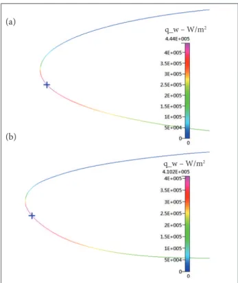
Figure 9 shows the heat flux distribution of the upper and lower surfaces of both airfoils. he maximum heat lux is reduced for the optimal case.

he optimized variables were also input to perform the CFD analysis. As shown in Table 3, the relative error between the RSM and CFD results is very small, which indicates that the surrogate model has a fairly good accuracy. he heat lux contours of the baseline and optimal airfoils are shown in Fig. 10, where the stagnation point positions are also marked.

Figure 9. Heat lux distribution of baseline and optimal airfoils.

Table 3. Optimization results.

Parameters Baseline Optimal Increment

(%)

Forecast error (%)

RSM CFD

Hypersonic condition q (W/m

2_{) 444,011 411,252 410,236 −7.61 0.25}

T (K) 1,768.7 1,734.8 1,734.0 −1.96 0.05

Landing condition

C_l 1.45276 1.46372 1.45905 0.43 0.05

C_d 0.04244 0.04219 0.04252 0.19 −0.78

K 34.23091 34.69353 34.31444 0.24 1.10

0.00 –0.09

0.09 Baseline

Optimal

–0.06 0.06

–0.03 0.03

0.00

0.05 0.10 0.15 0.20 0.25

x/c

y

/

c

x/c

0.0 0 1 2 3 4 5 × 105

Baseline Optimal

0.2 0.4 0.6 0.8 1.0

q

[W/m

2]

q_w – W/m2

q_w – W/m2

Figure 8. Shape of baseline and optimal airfoils.

Figure 10. Heat lux contours of airfoil leading edge. (a) Baseline; (b) Optimal.

(a)

J. Aerosp. Technol. Manag., São José dos Campos, Vol.9, No _{4, pp.503-509, Oct.-Dec., 2017}

CONCLUSION

An aerothermodynamic optimization procedure consi- dering the landing aerodynamic performance has been developed for NACA 0012 airfoil. In the optimization study, a modified Hicks-Henne type function is first adopted to parametrically describe the airfoil leading edge. CFD models are then established and further validated to simulate the hypersonic and landing problem. An optimization approach composed of DOE, RSM and MIGA is us ed to obtain the optimal air f o il. It is found that the surrogate model results agree well with the CFD ones. The optimal airfoil has a lower peak heat flux at the stagnation point compared with the baseline one. M eanwhile, the lift-to-drag ratio at landing condition is nearly the same as that of the baseline airfoil.

ACKNOWLEDGEMENTS

his study was supported by the Funding of Jiangsu Innovation Program for Gr ad u ate Education (Grant No. CXLX13_163), the

Fundamental Research Funds forthe Central Universities (Grant No. NZ2016101) and a project funded by the Priority Academic Program Development of Jiangsu Higher Education Institutions (PAPD).

AUTHOR’S CONTRIBUTION

Conceptualization, Wang Z and Kretov A; Methodology, Zhou C and Zhi J; Investigation, Zhou C and Zhi J; Writing – Original Drat, Zhou C, Zhi J and Kretov A; Writing – Review & Editing, Zhou C and Wang Z; Funding Acquisition, Wang Z; Resources, Wang Z; Supervision, Wang Z and Kretov A.

REFERENCES

Allen HJ, Eggers Jr AJ (1958) A study of the motion and aerodynamic heating of ballistic missiles entering the Earth’s atmosphere at high supersonic speeds. NACA-TR-1381. Washington: NACA.

Bian Y, Zhong J (1986) Heat transfer of high temperature boundary layer. Beijing: Science Press. In Chinese.

Buckley HP, Zingg DW (2013) Approach to aerodynamic design through numerical optimization. AIAA J 51(8):1972-1981. doi: 10.2514/1.J052268

Dassault Systèmes Simulia Corp. (2012) Isight 5.7 User’s Guide. Providence: Dassault Systèmes Simulia Corp.

Hicks RM, Henne PA (1978) Wing design by numerical optimization. J Aircraft 15(7):407-412. doi: 10.2514/3.58379

Koziel S, Leifsson LT (2014) Multi-objective airfoil design using variable-idelity CFD simulations and response surface surrogates. AIAA 2014-0289. Proceedings of the 10th AIAA Multidisciplinary Design Optimization Conference; National Harbor: USA.

Ladson CL (1988) Effects of independent variation of Mach and Reynolds numbers on the low-speed aerodynamic characteristics of the NACA 0012 airfoil section. NASA-TM-4074. Washington: NASA.

Launius RD, Jenkins DR (2012) Coming home: reentry and recovery from space. Washington: National Aeronautics and Space Administration.

Li P, Zhang B, Chen Y (2012) An effective transonic airfoil optimization method using Response Surface Model (RSM). Journal of Northwestern Polytechnical University 3:395-401. In Chinese.

Liem RP, Mader CA, Martins JRRA (2015) Surrogate models and mixtures of experts in aerodynamic performance prediction for aircraft mission analysis. Aerosp Sci Technol 43:126-151. doi: 10.1016/j.ast.2015.02.019

Lu Z (2009) Aerodynamics. Beijing: Beihang University Press. In Chinese.

McKay MD, Beckman RJ, Conover WJ (1979) A comparison of three

methods for selecting values of input variables in the analysis of output from a computer code. Technometrics 21(2):239-245. doi: 10.2307/1268522

Park C, Joh C, Kim Y (2009) Multidisciplinary design optimization of a structurally nonlinear aircraft wing via parametric modeling. Int J Precis Eng Man 10(2):87-96. doi: 10.1007/s12541-009-0032-1

Powers BG (1986) Space Shuttle longitudinal landing lying qualities. J Guid Contr Dynam 9(5):566-572. doi: 10.2514/3.20147

Rochelle WC, Roberts BB, D’Attorre L, Bilyk MA (1973) Shuttle orbiter re-entry lowields at high angle of attack. J Spacecraft Rockets 10(12):783-789. doi: 10.2514/3.61969

Sellers JJ (2004) Understanding space: an introduction to astronautics. New York: McGraw-Hill.

Sun R, Chen G, Zhou C, Zhou LW, Jiang JH (2013) Multidisciplinary design optimization of adaptive wing leading edge. Sci China Technol Sci 56(7):1790-1797. doi: 10.1007/s11431-013-5250-1

Tetzman DG (2010) Simulation and optimization of spacecraft re-entry trajectories (Master’s thesis). Minneapolis: University of Minnesota.

Wang YZ, Li F, Zhang X, (2015) Composite wind turbine blade aerodynamic and structural integrated design optimization based on RBF Meta-Model. Materials Science Forum 813:10-18. doi: 10.4028/www.scientiic.net/MSF.813.10

Xia C, Chen W (2015) Gradient-based aerothermodynamic optimization of a hypersonic wing proile. Procedia Engineering 126:189-193. doi: 10.1016/j.proeng.2015.11.214

Yang B, Xu Q, He L, Zhao LH, Gu CG, Ren P (2015) A novel global optimization algorithm and its application to airfoil optimization. Journal of Turbomachinery 137(4):041011. doi: 10.1115/1.4028712