J. Aerosp. Technol. Manag. vol.9 número4 jatm v9i4727

(1)

J. Aerosp. Technol. Manag., São José dos Campos, Vol.9, No_{4, pp.489-494, Oct.-Dec., 2017} ABSTRACT: Using the mathematical apparatus of the extended

Kalman Filter, the recurrent algorithm of the passive location in sensor networks — based on the Time Difference of Arrival method in case of correlated errors of measurements — is developed. The initial estimates of Radio Frequency Sources coordinates and the correlation matrix of the vector estimation are determined based on the method of the least squares in case of 3 difference measurement distances. Eficiency analysis of recurrent adaptive algorithm and its comparison with the quadratic correction one are performed by statistical modeling. A comparison of them with the lower limit of the Cramer-Rao was carried out. The implementation of the recurrent adaptive algorithm requires 2.7 times less computational cost than the quadratic correction one.

KEYWORDS: Passive location, Time Difference of Arrival method, Extended Kalman Filter, Recurrent adaptive algorithm, Sensor network.

Recurrent Algorithm for TDOA Localization

in Sensor Networks

Igor Olegovych Tovkach1_{, Serhii Yakovych Zhuk}1

INTRODUCTION

he problem of passive position determination of Radio Frequency Sources (RFS) is widely met in the monitoring of the surrounding space, disaster management, in intelligent transport and security systems. Currently, sensor networks are used for its solution (Rullan-Lara et al. 2013; Amar and Leus 2010).

One of the main approaches of passive position determination of RFS is based on the application of the Time Diference of Arrival method (TDOA), which uses the time diference of reception of signals received by the various sensors and the network reference sensor. his method has a signiicant advantage in the ease of implementation, being widely used in practice ITU (2014). he accuracy of determining the RFS coordinates based on the TDOA depends on the errors from measuring time signal reception sensors of the sensor network. he errors from the determination of the diference in signal reception times are correlated, because they contain the error in the reference sensor measurement.

In the known methods for determining the RFS coordinates based on the TDOA (Buzuverov 2008), the coordinate calculation is performed after receiving the measurements from all sensors. In this study, based on the mathematical apparatus of the extended Kalman Filter, the algorithm is developed, which — ater the formulation of the initial conditions based on the measurement of time for receiving signals from 4 sensors — allows to recurrently specify the location of RFS as the measurement proceeds from the other sensors. he developed algorithm also evaluates the time error from receiving the signal by the reference sensor measurement that allows considering the synthesized algorithm as adaptive.

1.National Technical University of Ukraine – Kyiv Polytechnic Institute – Department of Radio Engineering Devices and Systems – Kyiv – Ukraine.

Author for correspondence: Igor Olegovich Tovkach | National Technical University of Ukraine – Kyiv Polytechnic Institute – Department of Radio Engineering Devices and Systems | Politekhnichna St. 12 | 03056 – Kyiv – Ukraine | Email: [email protected]

(2)

J. Aerosp. Technol. Manag., São José dos Campos, Vol.9, No_{4, pp.489-494, Oct.-Dec., 2017} 490 Tovkach IO, Zhuk SYa

FORMULATION OF THE PROBLEM

The sensors network transducers have the coordinates (x S

i , y S

i ), i = 0, n. he position of the RFS is characterized by a point with coordinates (x, y). When determining the coordinates

of RFS on the x-y plane, the sensor network should consist

of no less than 4 sensors. Figure 1 shows block diagrams of sensor networks on the x-y plane, consisting of 9 (n = 8) and

4 (n = 3) sensors.

When using TDOA, the time diference in the reception of signals between the sensors i = 1, n and the reference probes

is measured:

distances v_i0, i = 1,n , are correlated because they contain the

reference sensor measurement error v₀.

he presence of correlated errors makes it diicult to use traditional recurrent target coordinates evaluation algorithms. his diiculty can be avoided through the introduction of v₀

into the state vector of the estimated parameters.

It is believed that, during the diference measurement of the distances between the RFS and the network sensors, its coordinates do not change. Synthesizing a recurrent algorithm is required, and, ater the formation of the initial conditions based on the measurement of signals receiving time from 4 sensors, it allows to specify recurrently the location RFS in process of receipt of measurements from the other sensors and to estimate the error of the reference sensor measurement.

DEVELOPMENT

The coordinates of the RFS position (x_k, y_k) should be

assessed; the measurement time of distance diference between the RFS and the network sensors, as well as its coordinates, do not change. he error in measurements of the reference sensor from Eq. 2 does not change as well in 1 measurement cycle, so the equation describing the dynamics of the estimated parameters has the form

(1) (2) (3) (4) (5) (6) (7)

where: t_i is the time of signal reception of the i − m sensor; t₀is the time of signal reception by the reference sensor; n_i is

the uncorrelated error of time measurements of signal by the reception of the i − m sensor (Buzuverov 2008) with dispersion σ 2 _n, i = 0, n.

Because of the transformation in Eq. 1, the TDOA equations for network can be represented as:

0 0 0

i

t

i

t

n

i

n

Δ

=

−

+

−

i

₌

1,

n

− −

n

−

)

−

₌

−

0

v

−

v

0

i

=

1,

n

x

y

−

+

1

k k

u

₋

k

v

k

=

+

−

+

−

ˆ

σ

− − − − − −   ∂ ∂ ∂ ⋅ _ _ ∂ _ ∂ ∂ _

ˆ

−



_

−



_

ˆ

_ˆ

P

− − −

∂

−

∂

ˆ

− − − − − − − − − − − − −

∂

−



−



∂

_

_

₋

_

_

−

₋

1

_A

1

_b

ω

_Σ

− −

_Σ

−

Δ

−

i0

=

+

n

−

(

)

−

₀

+

n

0

−

(

)

0

v

=

−

+

−

0

v

−

v

0

i

=

1,

n

y

−

1

k k

u

₋

k k

=

+

y

−

ˆ ˆ

_σ

− − − − − −   ∂ ∂ ∂ ⋅   ∂ _ ∂ ∂ _ −



_

−



_

ˆ

₋

_ˆ

− −

∂

−

∂

ˆ

− − − − − − − − − − − − −





∂

−



−



∂

_

_

₋

_

_

−

₋

1

_A

1

ω

_Σ

− −

_Σ

−

Δ

−

− −

n

−

)

0 0 0 0

,

1,

v

n

−

+

−

=

−

+

=

)

0

v

−

v

0

i

=

1,

n

y

−

+

1

k k

u

₋

k k

=

+

−

1

σ

− − − − − −   ∂ ∂ ∂ ⋅ _ _ ∂ _ ∂ ∂ _

ˆ

−



_

−



_

ˆ

₋

_ˆ

− −

∂

−

∂

ˆ

− − − − − − − − − − − − −



∂

−



−



∂



_

−



_

−

₋

1

_A

1

_b

ω

_Σ

− −

_Σ

−

Δ

−

− −

−

0 0

v

₌

v

−

v

i

₌

_1,

n

y

−

+

1

k k

u

₋

k k

=

+

y

−

+

−

ˆ

σ

− − − − − −   ∂ ∂ ∂ ⋅   ∂ _ ∂ ∂ _

ˆ

−



_

−



_

ˆ

₋

_ˆ

− −

∂

−

∂

ˆ

− − − − − − − − − − − − −



∂

−



−



∂

_

_

₋

_

_

−

₋

1

_A

1

_b

ω

_Σ

− −

_Σ

−

Δ

−

− −

−

S S

0

)

R

−

R

=

−

+

y

−

y

−

+

y

1

k k

u

₋

)

k k

=

+

y

−

ˆ

σ

− − − − − −   ∂ ∂ ∂ ⋅ _ _ ∂ _ ∂ ∂ _

ˆ

−



_

−



_

ˆ

₋

_ˆ

− −

∂

−

∂

S

ˆ

− − − − − − − − − − − − −



∂

−



−



∂

_

_

₋

_

_

−

₋

1

_A

1

_b

ω

_Σ

− −

_Σ

−

Δ

−

− −

−

1

k k

u

=

u

₋

k k

=

+

)

y

−

+

−

ˆ

σ

− − − − − −   ∂ ∂ ∂ ⋅ _ _ ∂ _ ∂ ∂ _

ˆ

−



_

−



_

ˆ

₋

_ˆ

− −

∂

−

∂

ˆ

− − − − − − − − − − − − −



∂

−



−



∂

_

_

₋

_

_

−

₋

1

_A

1

_b

ω

Σ

− −

Σ

−

Δ

−

− −

−

k

=

k

+

k

)

y

−

+

−

ˆ

ˆ ˆ

_σ

− − − − − −   ∂ ∂ ∂ ⋅ _ _ ∂ _ ∂ ∂ _

ˆ

−



_

−



_

ˆ

₋

_ˆ

− −

∂

−

∂

ˆ

− − − − − − − − − − − − −



∂

−



−



∂



_

−



_

−

₋

1

_A

1

_b

ω

_Σ

− −

_Σ

−

Δ

−

− −

−

− 0

)

k k

y

k

y

k

y

k k

=

−

+

−

+

−

;

1

σ

− − − − − −   ∂ ∂ ∂ ⋅ _ _ ∂ _ ∂ ∂ _

ˆ

−



_

−



_

ˆ

₋

_ˆ

− −

∂

−

∂

S

ˆ

− − − − − − − − − − − − −



∂

−



−



∂

_

_

₋

_

_

−

₋

1

_A

1

_b

ω

_Σ

− −

_Σ

−

where: R_i is the distance between the i − m sensor and the RFS, i = 1, n; R₀ is the distance between the reference sensor and

the RFS; d_i0 is the measured diference of distances i = 1, n; c is the spreading speed of electromagnetic waves; t is the

moment of RFS signal emission; v_i0 is the error of diference

measurement between the distances:

where: v_i are the uncorrelated random variables having

the meaning of the distance measurement errors between the RFS and the network sensors with a dispersion σ 2 _v = c 2σ 2 _n , i = 0, n.

he diference in distance R_i – R₀ is determined by the formula

In Eq. 4, the coordinates of the reference sensor were relied to be 0. he errors of diference measurement between the

where: u_k = (x_k, y_k, v_0k)T_{is the state vector including position} coordinates of the RFS and the measurement error of the reference sensor v_0k on the current time step k. he index k

characterizes the incomings sequence of measured diferences in distances.

he measurement equation describing the measured kth

distance diference considering Eqs. 2, 4 and 5 can be viewed as

where: h(u_k) is a linear function described by the

non-linear measurement expression:

(3)

J. Aerosp. Technol. Manag., São José dos Campos, Vol.9, No_{4, pp.489-494, Oct.-Dec., 2017} 491

Recurrent Algorithm for TDOA Localization in Sensor Networks

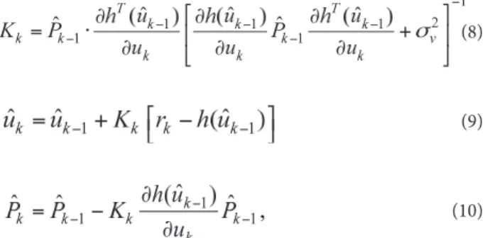
Using the model (Eqs. 6 and 7), a recurrent estimation algorithm of the state vector can be obtained based on the extended Kalman Filter (Welch and Bishop 2006), being described by

he correlation matrix Ω of the vector estimation error ω

is deined (Amar and Leus 2010) by

(12) (13) ...continue (11) (8) (9) (14) (15) (10)

− −

−

1 2

1 1 1

1 1

ˆ ˆ ˆ

ˆ ˆ

T T

v

K P P

σ

− − − − − −   ∂ ∂ ∂ = ⋅ _ + _

∂ _ ∂ ∂ _

8)

ˆ

h u

−



_

−



_

;

)

ˆ

₋

_ˆ

− −

∂

−

∂

S

ˆ

− − − − − − − − − − − − −



∂

−



−



∂



_

−



_

−

₋

1

_A

1

_b

ω

_Σ

− −

_Σ

−

− −

−

σ

− − − − − −   ∂ ∂ ∂ ⋅ _ _ ∂ _ ∂ ∂ _ 1 1

ˆ

u

r

h u

−



−



=

+

_

−

_

;

ˆ

h u

−

ˆ

− −

∂

−

∂

,

ˆ

− − − − − − − − − − − − −



∂

−



−



∂

_

_

₋

_

_

−

₋

1

_A

1

_b

ω

Σ

− −

Σ

−

− −

−

σ

− − − − − −   ∂ ∂ ∂ ⋅   ∂ _ ∂ ∂ _ −



_

−



_

1 1 1

ˆ

h u

u

− − −

∂

=

−

∂

,

ˆ

− − − − − − − − − − − − −



∂

−



−



∂

_

_

₋

_

_

−

₋

1

_A

1

_b

ω

_Σ

− −

_Σ

−

Δ

−

− −

−

σ

− − − − − −   ∂ ∂ ∂ ⋅ _ _ ∂ _ ∂ ∂ _ −



_

−



_

− − −

∂

−

∂

1 1 1 1

ˆ

)

ˆ

h u

u

− − − − − − − − − − − − −



∂

−



=

−

∂



_

−

+

−



_

−

₋

(

A

ω

_Σ

− −

_Σ

−

Δ

−

− −

−

σ

− − − − − −   ∂ ∂ ∂ ⋅ _ _ ∂ _ ∂ ∂ _ −



_

−



_

− − −

∂

−

∂

S 1 1

1 1 1 1

ˆ

;

ˆ

)

ˆ

− − − − − − − − − − − − −



∂

−



−



∂



_

−

+

−

+

−



_

−

₋

1

_A

1

_b

ω

_Σ

− −

_Σ

−

Δ

−

− −

−

σ

− − − − − −   ∂ ∂ ∂ ⋅   ∂ _ ∂ ∂ _ −



_

−



_

− − −

∂

−

∂

1 1 1

ˆ

)

ˆ

; 1

− − − − − − − − − − − − −



∂

−



−



∂

_

_

₋

+

_

_

−

₋

1

_A

1

_b

ω

Σ

− −

Σ

−

Δ

−

− −

−

σ

− − − − − −   ∂ ∂ ∂ ⋅ _ _ ∂ _ ∂ ∂ _ −



_

−



_

− − −

∂

−

∂

− − − − − − − − − − − − −



∂

−



−



∂

_

_

₋

_

_

−

₋

(

₁

)

1 ₁

b

A

ω

₌

_Σ

− −

_Σ

−

_,

where: u ˆ_k is the estimation of the state vector u_kat the kth step; P ˆ_k is the correlation matrix of the state vector of the estimation

error u_k at the kth step; K_k is the coeicient of the ilter gain:

he resulting algorithm (Eqs. 8 – 10) is non-linear and belongs to the class of the adaptive ones because it along with the estimation of the RFS the coordinates, an estimation of the unknown error v₀ is determined. he initial conditions

of u ˆ₀ and P ˆ₀ must be set for the implementation of adaptive

iltering. he initial evaluation of the vector u ˆT ₀ is u ˆT ₀=(x ˆ₀, y ˆ₀, 0)

he initial estimates of RFS coordinates x ˆ₀, y ˆ₀ are determined

based on the method of least squares (LS) in case of 3 diference measurement distances (Amar and Leus 2010) using the Eq. 12:

where: ωT₌₍_x_ˆ

0, y ˆ0, R ˆ0) is the vector consisting of the RFS assessment;

S S 1 1 10 S S

S S

3 3 3

x y d

A

=

− − −

σ σ σ

 

 

Σ  

      1 A A − −  

Ω _ Η _

 

) ;j 1,3

− − = ˆ P ˆ σ × Ω

 Ω× Ω

y d S S

1 1 10 S S

S S

3 3 30 x y x + − = + − + −

σ σ σ

 

 

Σ  

      1 A A − −  

Ω _ Η _

 

) ;j 1,3

− − = ˆ P 0 σ × Ω

 Ω× Ω

− − −

σ σ σ

 

 

Σ=_ _

      1 A A − −  

Ω _ Η _

 

) ;j 1,3

− − = ˆ P 0 σ × Ω

 Ω× Ω

− − −

σ σ σ

 

 

Σ  

 

 

( )

0 ₁ 0 1

A A

− −

 

Ω=_ Η _

  ,

) ;j 1,3

− − = ˆ P ˆ σ × Ω

 Ω× Ω

− − −

σ σ σ

 

 

Σ  

      − −  

Ω _ Η _

  − − ˆ P 0 0 ˆ 0 σ × Ω = 

Ω× Ω

where: H is the matrix determined by the formula H = B∑B;

B = diag {R ˆ₁, R ˆ₂,R ˆ₃}; R ˆ_j= √(x ˆ₀– x S

0 )2 + (y ˆ0 – y S 0 )2; j = 1, 3. he initial correlation matrix P ˆ₀ has the block form

where Ω_2×2 is determi 56’[p-;;;;;;n 56734r5 ned based on Ω, by deleting the third row and the third column.

Ater the formation of the initial conditions based on the time measurements to receive signals from the 4 sensors, the synthesized algorithm (Eqs. 8 – 10) allows to recurrently specify, at each step k, the location of the RFS as the measurement

proceeds from the other sensors k = 1, n – 3.

THE EFFECTIVENESS OF THE

ALGORITHM ANALYSIS

The efficiency analysis of recurrent adaptive algorithm (Eqs. 8 – 10) and its comparison with the quadratic correction one is performed by statistical modeling. he quadratic correction algorithm provides the highest accuracy among those considered in Amar and Leus (2010). It consists of 2 stages: (i) evaluate the RFS coordinates, which depends on the distance R₀_,substitute

in the initial functionality then re-solve the linear optimization problem; (ii)–adjust the solution for a quadratic relation.

he modeling of algorithms is performed for the sensor network coniguration (Fig. 1a), which consists of 9 sensors to determine the RFS position at the coordinates: S0(0; 0), S1(0; 20), S2(20√2; 20√2), S3(20; 0), S4(20√2; –20√2), S5(0; −20), S6(–20√2; –20√2), S7(−20; 0) and S8(–20√2; 20√2). Figure 1b shows a sensor network with a minimal number of sensors to form the initial adaptive iltering conditions with the coordinates: S0(0; 0), S1(20√2; 20√2), S2(20√2; –20√2) and S3(−20; 0). he RFS is placed on a circle with a radius of 100 km relative to the reference sensor D₀. he root mean

(4)

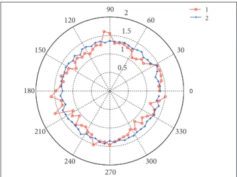
Figure 2. Circular RMS of the RFS position estimation error for the initial conditions.

Figure 1. Coniguration of the sensor network with (a) 9 and (b) 4 sensors.

Figure 3. Circular RMS of the RFS position estimation error for recurrent adaptive algorithm.

Y

Y y

y S₁

S₁ S8

S₇ _S

0

S0 S2

S2 S₆

S5 S4 S3

S3

r6 r7

r8 r1

r1 r2

r3

r2 r4 r5

r3 r

r

x

X

X RFS

RFS

2

4 6

8

30

210

60

240

90

270 120

300 150

330

180 0

1 2

0.5 1

1.5 2

30

210

60

240

90

270 120

300 150

330

180 0

1

2

( a )

( b )

s q u a re (RMS) of the measurement error is s_v = 30 m. As an

indicator of the eiciency, the circular standard deviation was used,σ ˆ = √σ ˆ 2 _x+ σ ˆ 2 _y

.

Figure 2 shows the dependence of the actual σ ˆ MC_LS (curve 1)

circular RMS of the RFS position estimation error with 4 sensors (Fig. 1b) obtained by Monte Carlo simulation using

Eq. 12, which corresponds to the initial conditions of the adaptive ilter. his igure also shows the dependence of the theoretical (curve 2) circular RMS of the RFS position estimation error, which is calculated based on relevant elements of the correlation matrix of estimation errors determined using Eq. 14. RMS values σ ˆ MC_LS range from 2 to 8 km.

Figure 3 shows the dependence of the actual σ ˆ MC_FK_{(curve 1)}

and theoretical σ ˆ_FK_{(curve 2) circular RMS of the RFS position}

estimation error with 9 sensors (Fig. 1) for the recurrent algorithm. he received actual and theoretical RMS values correspond well, indicating the proper operation of the algorithm. MSE values σ ˆ MC_FK range from 1.3 to 1.9 km. he application of

recurrent adaptive algorithm reduces the circular RMS of the RFS location estimation error in 1.5 – 4.2 times (Fig. 3).

Figure 4 shows the dependence of the actual σ ˆ MC_QC (curve 1;

where QC is the quadratic correction) and theoretical σ ˆ_FK (curve 2)

circular RMS of the RFS location estimation error for the quadratic correction algorithm.

Figure 5 shows a circular RMS of the RFS location estimation error, which corresponds to the lower limit of the Cramér-Rao bound and characterizes the potential accuracy of the possible RFS coordinates. he values of circular RMS error of the RFS positioning of the recurrent adaptive and quadratic correction algorithms, positioned close to the corresponding values of circular RMS of the Cramér-Rao bound lower limit, indicate their high eiciency.

(5)

J. Aerosp. Technol. Manag., São José dos Campos, Vol.9, No_{4, pp.489-494, Oct.-Dec., 2017}

Figure 4. Circular RMS of the RFS position estimation error for the quadratic correction algorithm.

0.5 1 1.5

2

30

210

60

240

90

270 120

300 150

330

180 0

1 2

RMS e

rr

o

r es

tima

ti

o

n o

f RFS

lo

c

a

ti

o

ns [k

m]

Sensors

0 0

0.5 0.5

1 1.5 2 2.5 3 3.5

1.5 2 2.5 3 3.5 4 4.5 5

1 2

0.5 1 1.5

2

30

210

60

240

90

270 120

300 150

330

180 0

1

Figure 6. Circular RMS dynamics of the RFS locations estimation error under sequential data arrival.

Figure 5. Circular RMS of the RFS position estimation error of the Cramér-Rao bound lower limit.

c o ordinates (x, y). he use of recurrent adaptive algorithm

reduces the circular RMS of the RFS location estimation error in 2.5 times relative to the initial conditions.

It is interesting to compare the calculation of the costs required in the implementation of the recurrent adaptive and quadratic correction algorithms. hey can be assessed by determining the number of required multiplications (divisions), since they are performed from 100 to 150 times slower than addition and subtraction. For the example with the implementation of the recurrent adaptive algorithm, 461 multiplications are required and, for the quadratic correction one, this value is 1,246. hus, the application of the developed algorithm reduces the computational cost by 2.7 times.

CONCLUSIONS

Using the mathematical apparatus of Kalman filtering, the algorithm is developed, which, after the formation of the initial conditions, is based on measurements of the receiving time of the signals from 4 sensors. This allows specifying the location of the recurrent RFS as the measurement proceeds from the other sensors. It belongs to the class of adaptive algorithms, because, along with the estimation of the RFS coordinates, it determines the estimation of unknown error of reference sensor measurement. According to the simulation results, the use of recurrent algorithm can reduce the circular RMS of the RFS location estimation error by 1.5 – 4.2 times, providing characteristics similar to the potentially achievable. he implementation of the recurrent adaptive algorithm requires 2.7 times less computational cost than the quadratic correction one. The resulting algorithm can also be easily extended to the case of RFS iltering trajectory at which its motion parameters are estimated (Chiang et al. 2012).

AUTHOR’S CONTRIBUTION

(6)

REFERENCES

International Telecommunication Union (2015) Comparison of methods of determining the geographic location of the signal source based on the time difference of arrival and angle of arrival of the signal Report ITU-R SM.2211-1. Geneva: ITU.

Amar A, Leus G (2010) A reference-free time difference of arrival source localization using a passive sensor array. Proceedings of the IEEE Sensor Array and Multichannel Signal Processing Workshop; Jerusalem, Israel.

Buzuverov GV (2008) Algorithms for passive location in a distributed network of sensors for the time difference of arrival method. In: Buzuverov GV, Gerasimov OI, editors. Information-measuring and control systems. Moscow: Radio Engineering.

Chiang CT, Tseng PH, Feng KT (2012) Hybrid Uniﬁed Kalman Tracking Algorithms for heterogeneous wireless location systems. IEEE Trans Veh Technol 61(2):702-715. doi: 10.1109/TVT.2011.2180939.

Rullan-Lara JL, Sanahuja G, Lozano R, Salazar S, Garcia-Hernandez R, Ruz-Hernandez JA (2013) Indoor localization of a quadrotor based on WSN: a real-time application. Int J Adv Robotic Sy 10(1):1-9. doi: 10.5772/53748.