Copyright © 2007 SBMAC ISSN 0101-8205
www.scielo.br/cam
On a convective condition in the diffusion of a
solvent into a polymer
MARCOS GAUDIANO1, TOMÁS GODOY2 and CRISTINA TURNER1,2 1FAMAF-UNC-CIEM-CONICET
2FAMAF-UNC. Córdoba, Argentina
E-mails: [email protected] / [email protected] / [email protected]
Abstract. We studied a one-dimensional free boundary problem arising in the polymer industry, which solution has an interesting asymptotic behavior when a convective boundary condition is imposed. We show the asymptotic behavior of the free boundary and of the concentration of the solvent in the domain, for larget. Exact estimates and numerical results are obtained.
Mathematical subject classification: 35K05, 35K60.
Key words: free boundary problems, diffusion, convective case, asymptotic behavior.
1 Introduction
In this paper we consider a free boundary problem arising from a model for sorption of solvents into glassy polymers.
This model was proposed in[1]by Astarita and Sarti. They assumed that the sorption process can be described using a free boundary model to simulate a sharp morphological discontinuity observed in the material between a penetrated zone, with a relatively high solvent content, and an glassy region where the solvent concentration is negligibly small (and actually taken to be zero in the model).
The solvent is supposed to diffuse in the penetrated zone according to Fick’s law. Moreover the penetrating zone moves into the glassy zone driven by chemi-cal and mechanichemi-cal effects that are taken into account by an empirichemi-cal law relating the speed of penetration to the concentration of solvent near the front. This law
must account for two main facts observed in the penetration experiences: (i) there exists a threshold value for the solvent concentration under which no pen-etration occurs; (ii) above such value the speed of the front increases with the concentration near the front itself. A typical form isv = α|u −q|m wherev
is the front speed,u is the value of the concentration at the front,q >0 is the
threshold value andαandmare positive constants ([1]).
An additional condition on the free boundary is obtained imposing mass servation, i.e., equating the mass density current to the product of solvent con-centration and the velocity of the free boundary.
This model has been the object of a number of papers. In [2], it has been studied with the condition of constant concentration at the boundary. In [3], it has been investigated assuming that the polymer is in perfect contact with a well-stirred bath. In [4], its authors were interested in the case of a slab of non-homogeneous polymer. In [5], it has been studied assuming a flux condition at the fixed boundary. Here we are interested in a convective case, where it is supposed that there is a flux of solvent through the left side of a slab proportional to the difference between the solvent concentration at x = 0 and a given function
of the time which represents an external solvent concentration (h > 0 is the
proportionality constant). Denoting byc(x,t)the normalized concentration and
byx =s(t)the location of the front in the slab the mathematical problem can
be stated as follows:
Problem PS. Find a triple (T,s,c) such that: T > 0, s ∈ C1[0,T], c ∈ C2,1(D
T)∩C(D¯T), where DT = {(x,t): 0 < t < T,0 < x < s(t)}, and
satisfying
cx x −ct = 0 in DT, (1.1)
cx(0,t) = h
c(0,t)−g(t), g(0) = 1, 0≤t≤T (1.2) ˙
s(t) = f(c(s(t),t)), 0≤t ≤T (1.3)
cx(s(t),t) = −˙s(t)
c(s(t),t)+q, 0≤t≤T (1.4)
s(0) = 0. (1.5)
The functiong(t)is positive and the quantityq+g(t)represents the external
∀T > 0, g′(t) ≤ 0 and G ≡ ∞
0 g(t)dt < ∞. Throughout the paper the
function f will be supposed to satisfy f ∈ C1(0,1], f′(c) > 0 forc ∈ (0,1]
and f(0) =0 (empirically, the function f is observed to be a power law). We
note that there exists= f−1which has the same properties as f.
2 Existence and some global estimates
Equating(1.2)to(1.4)fort=0, we have thatc∗=. c(0,0)is the unique solution
of f(c∗)(c∗+q)= −h(c∗−1). The solution satisfies 0<c∗<1.
The existence forPSis accomplished as follows: Letr ∈C1[0,T] ∩C2(0,T)
be such that
r(0) = 0, (2.6)
˙
r(0) = f(c∗), (2.7)
0 ≤ ˙r(t) ≤ f(c∗) in [0,T], (2.8)
|¨r(t)| ≤ K in (0,T), (2.9)
and consider the problem (PA) of findingc ∈ C2,1(D)
∩C(D¯),cx continuous up tox =r(t),t ∈(0,T), such that
cx x−ct = 0 in D =
(x,t):0<t<T,0<x <r(t), (2.10)
cx(0,t) = h
c(0,t)−g(t), g(0) = 1, 0≤t ≤T, (2.11)
cx(r(t),t) = −˙r(t)
(r˙(t))+q
, 0≤t ≤T. (2.12)
Thus, we note thatPAdiffers fromPSby the fact that the curver(t)is given.
In [7], it is shown that the transformation
r(t)→ t
0
f(c(r(t),t)), 0<t <T, (2.13)
has a unique fixed point forT >0 small enough, which is actually the desired
curves(t)ofPS. The global existence and uniqueness forPSis also established in [7]. Now we prove:
Proposition 2.1. Assumes,csolve problemPSfor a givenT <+∞. Then
0<c(x,t) <1 0≤ x ≤s(t), t ≥0, (2.14)
Proof. Using the Hopf’s lemma we can assume that c attains its maximum
value on x = 0 since cx = −f(c)((s˙) +q) ≤ 0 on x = s(t). Let be
c(0,t0) =maxDTc. Ift0 = 0, then maxDT c = c∗ < 1. Otherwise we have 0 > cx(0,t0)= h(c(0,t0)−g(t0)), which implies maxDTc < g(t0) ≤ 1. Let
bec(x1,t1) = minDTc. If x1 = 0 then there occurs either minDT c =c∗ >0 or minDT c = g(t1)+1/(h)cx(0,t1) ≥ g(t1) > 0. Moreover, if minDT c =
c(s(t1),t1)=0 (witht1>0) thencx(s(t1),t1)=0, contradicting the boundary
point principle. Thus,(2.14)holds andcx(0,t) <h(1−g(t))for allt. Finally, let us suppose that minDT cx =cx(s(t2),t2)witht2≥0. Ift2>0 then
0 ≥ d
dtcx(s(t),t)|t=t2, i.e.
0 ≤ −
f′(c(s(t2),t2))(c(s(t2),t2)+q)+ f(c(s(t2,t2)))
cx(s(t2),t2)s˙(t2)+cx x(s(t2),t2)
>0,
which is a contradiction. Then minDT cx =cx(0,0)=h(c∗−1).
Proposition 2.2. Under the assumptions above, the following estimate holds
|ct(x,t)| ≤ BT, ∀(x,t)∈ DT, (2.16)
with
BT = max
max
[0,T]|g
′|, f(1)2(1
+q),|ct(0,0)|
. (2.17)
Proof. Note from(1.2)that
ct(0,t) = g′(t)+ 1
hct x(0,t), 0<t ≤T. (2.18)
Moreover, from(1.3)and(1.4) we havecx = −f(c)(c+q)at x = s(t)and deriving with respect totwe get
ctf(c)+ct x = −
f′(c)(c+q)+ f(c) cxf(c)+ct
at x =s(t) (2.19)
ct(s(t),t)=
f′(c)(c+q)+ f(c) f2(c)(c+q)−ct x 2f(c)+ f′(c)(c+q)
x=s(t)
(2.20)
3 The numerical method
In this section will be shown a numerical scheme based on the method introduced in[6]for one-dimensional parabolic free boundary problems with arbitrary im-plicit or exim-plicit free boundary conditions.
In this method the continuous problem is time discretized and solved at succes-sive time levels as a sequence of free boundary problems for ordinary differential equations. Specifically, at time levelt = tn withtn −tn−1 = t the solution {Cn(x),Sn}is computed as the exact solution of the discretized equations
Cn′′−Cn−Cn−1
t = 0 0<x <Sn, (3.21)
Cn′(0) = h(Cn(0)−g(tn)) , (3.22)
Sn−Sn−1
t = f(Cn(Sn)), S0 = 0, (3.23)
Cn′(Sn) = −
Sn−Sn−1
t (q+Cn(Sn)). (3.24)
In(3.21)the function Cn−1(x)is supposed to be defined over[0,+∞), and Sn−1supposed to be known as well. We write(3.21)as a first order system over (0,Sn)
Cn′ = Vn, (3.25)
Vn′ = 1
t (Cn−Cn−1) (3.26)
and exploit the observation thatCnandVnare related through the Riccati trans-formation
Cn(x) = R(x)Vn(x)+Wn(x), (3.27) where
R(x) = √
t
tanhx+K
√
t
, K =
√
ttanh−1(h√t) (3.28)
Wn′ = −R(x)
t (Wn−Cn−1(x)) , Wn(0) = g(tn). (3.29)
Vn,Snsimultaneously satisfies(3.23),(3.24)and(3.27). Elimination ofCnand
Vnfrom(3.24)and(3.27)shows thatSnmust be a root of the scalar equation
σn(x)
.
= x −Sn−1
t − f
Wn(x)−q R(x)(x −Sn−1)/t
1+R(x)(x −Sn−1)/t
= 0. (3.30)
Given Sn, we set
Cn(Sn) =
Wn(Sn)−R(Sn)S˙nq 1+R(Sn)S˙n
, (3.31)
so that
˙ Sn
.
= Sn−Sn−1
t = f(Cn(Sn)) , (3.32)
and
Cn′(Sn) = Vn(Sn) = − ˙Sn
Wn(Sn)+q 1+R(Sn)S˙n
. (3.33)
Thus, the triple{Cn(Sn),Vn(Sn),Sn}is an exact solution of(3.23),(3.24)and
(3.27). We remark that depending ont the functionalσn(x)may have a root smaller than Sn−1. Such a root would correspond to a negative concentration Cn(Sn) and is not admissible. We shall therefore agree to choose for Sn the smallest root ofσn(x)=0 on(Sn−1,∞). Such a root will be soon to exist.
OnceSn has been determined, one can findVnby integrating backward over
[0,Sn)the equation
Vn′ = 1
t R(x)Vn+Wn(x)−Cn−1(x)
, (3.34)
withVn(Sn)given by(3.33). The concentrationCn(x)at time leveltnis obtained from (3.27). Finally, Cn(x) is extended over [Sn,∞) as C1 linear function, becauseCn+1(x)will be computed in[0,Sn+1], withSn+1>Sn,as the solution of an ODE depending onCn.For the initial concentration we shall use
C0(x) = −h(1−c∗)x+c∗.
Proof. We note thatC0(S0) =c∗ ∈(0,1)andC0′ = −h(1−c∗) <0. Let us
proceed by induction and assume the result valid forn−1. Integrating(3.29)
we have
Wn(x)= 1 sinhx+K
√
t
g(tn)sinh
K
√
t
+√1
t
x
0
cosh
r+K
√
t
Cn−1(r)dr
,
sinceCn−1<1 by assumption, we get
Wn(x)≤ 1 sinhx+K
√
t
g(tn)sinh
K
√
t
+√1
t
x
0
cosh
r+K
√ t dr , = 1
sinhx√+K t
g(tn)sinh
K √ t + sinh
x+K
√ t −sinh K √ t ≤1
moreoverWn(Sn−1) >0. Hence the function
Wn(x)−q R(x)(x −Sn−1)/t
1+R(x)(x −Sn−1)/t
is less than one and positive on some interval(Sn−1,x0), vanishing onx0. Then, σn(x0) =
x0−Sn−1
t − f(0) >0,
what is more
σn(Sn−1) = −f(Wn(Sn−1)) <0,
thus there must be a point Sn ∈ (Sn−1,x0)whereσn(Sn) =0, 0<Cn(Sn) < 1 andC′
n(Sn) <0. Integrating(3.27)we obtain: 0<Cn(x)
=cosh
x+K
√
t
Cn(Sn) coshSn+K
√ t − 1 √ t x Sn
sinhr√+K t
cosh2r+K
√
t
Wn(r)dr
≤cosh
x+K
√
t
Cn(Sn) coshSn+K
√ t − 1 √ t x Sn
sinhr√+K t
cosh2r+K
√
t
dr
=Cn(Sn)
coshx√+K t
coshSn+K
√
t
+1−
coshx√+K t
coshSn+K
√
t
Finally, from(3.31)and(3.32)we conclude thatSn−Sn−1= f(Cn(Sn))t <
f(1)t.
Remark. Sn−1can not be an accumulation point of the set of points that satisfy σn(x)=0 sinceσnis a continuous function andσn(Sn−1) <0.
4 Asymptotic behavior
In this section we show some results about the behavior of the free boundarys(t)
whent goes to infinity.
Lets(t),c(x,t)solve problemPS. Using Green’s identity we get:
0=
∂Dt
c(x,t)v(x,t)d x+(v(x,t)cx(x,t)−c(x,t)vx(x,t))dt t>0, (4.35)
which holds for every solutionv =v(x,t)ofvx x +vt =0 inDt. Thus, taking
v(x,t)=1 we obtain
0=
∂Dt
c(x,t)d x+cx(x,t)dt t >0,
which gives
0 =
t
0
c(s(τ ), τ )s˙(τ )dτ − t
0 ˙
s(τ ) (c(s(τ ), τ )+q) dτ
− s(t)
0
c(x,t)d x − t
0
cx(0, τ )dτ
and then
qs(t) = − s(t)
0
c(x,t)d x − t
0
cx(0, τ )dτ (4.36)
= − s(t)
0
c(x,t)d x −h t
0
c(0, τ )dτ +h t
0
g(τ )dτ (4.37)
so
s(t) ≤ h q
t
0
g(τ )dτ ≤ h
qG. (4.38)
This upper bound is independent of f, and sinces˙(t)= f(c(s(t),t)) >0 there
exists
s∞ =. lim
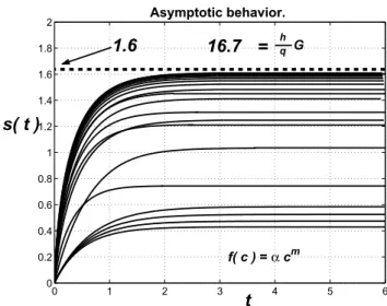
The following numerical result shows these facts for the caseq =.3,h =10, g(t) = e−2t and several functions f hqG = 16.7. We solved the equations (3.29)and(3.34)using Runge-Kutta method implemented in Matlab as ODE45,
with the step size and tolerance established by default.
0 1 2 3 4 5 6
0 0.2 0.4 0.6 0.8 1 1.2 1.4 1.6 1.8
2 Asymptotic behavior.
t s( t )
1.6
f( c ) = α cm
h q
= 16.7 G
Figure 1 – Plot of the free boundaries and their asymptotic behaviors for several func-tion f(c)=αcm,α >0,m>0.
The Figure 1 shows that all the free boundaries are bounded nearly by 1.6, so
h
qGappears to be a very large bound, and we can look for a better one. In order to do it, we will obtain two additional equations forsandc((4.40)and(4.41)
below). First, takingv(x,t)=xin(4.35)we have
0=
∂Dt
c(x,t)x d x+(xcx(x,t)−c(x,t)) dt,
it gives
0 =
t
0
c(s(τ ), τ )s(τ )s˙(τ )dτ
+ t
0
−(q+c(s(τ ), τ ))s˙(τ )s(τ )−c(s(τ ), τ )dτ
− s(t)
0
c(x,t)x d x+ t
0
q
2s
2(t) +
t
0
c(s(τ ), τ )dτ = − s(t)
0
c(x,t)x d x+ t
0
c(0, τ )dτ. (4.40)
Similarly, takingv(x,t)=t−x22 we get:
0=
∂Dt
c(x,t)
t−x 2
2
d x+
t− x
2
2
cx(x,t)+xc(x,t)
dt, thus 0 = 0 t
τcx(0, τ )dτ +
t
0
c(s(τ ), τ )
τ −s 2(τ )
2
˙ s(τ )
+
τ −s 2(τ )
2
cx(s(τ ), τ )+c(s(τ ), τ )s(τ )
dτ
+ 0
s(t) c(x,t)
t−x
2
2
d x,
and so
0 = −
t
0
τcx(0, τ )dτ −
q
6s
3(t) −q
t
0
τs˙(τ )dτ
+ t
0
c(s(τ ), τ )s(τ )dτ +1
2
s(t)
0
x2c(x,t)d x −t
s(t)
0
c(x,t)d x.
(4.41)
Lemma 4.1. The following equation holds:
lim t→∞
s(t)
0
c(x,t)d x =0. (4.42)
Proof. From(4.41)we have
s(t)
0
c(x,t)d x = −1 t
t
0
τcx(0, τ )dτ −
q
6ts 3
(t)−q t
t
0
τs˙(τ )dτ
+1 t
t
0
c(s(τ ), τ )s(τ )dτ + 1
2t s(t)
0
x2c(x,t)d x
≤ −1t t
0
τcx(0, τ )dτ+ 1
t t
0
c(s(τ ), τ )s(τ )dτ +s 3
∞
To prove the lemma it is enough that all these terms go to zero as t→ ∞. In
order to do it, note that from(4.37),
t
0
c(0, τ )dτ ≤ t
0
g(τ )dτ ≤G,
then, using(4.40)
t
0
c(s(τ ), τ )s(τ )dτ ≤s∞ t
0
c(s(τ ), τ )dτ ≤s∞G,
thus
lim t→∞
1
t t
0
c(s(τ ), τ )s(τ )dτ =0.
On the other hand, from(4.36)
− t
0
cx(0, τ )dτ =
s(t)
0
q+c(x,t)
d x >0 (4.43)
and from(1.2)
− ∞
0
cx(0, τ )dτ =h
G−
∞
0
c(0, τ )dτ
<∞. (4.44)
And integration by parts gives
lim t→∞
1
t t
0
τcx(0, τ )dτ
= tlim
→∞
t
0
cx(0, τ )dτ − 1
t t
0
τ
0
cx(0, τ′)dτ′
dτ
= 0.
Where in the last equality we have used(4.43),(4.44)and the L’Hôpital’s rule.
Lemma 4.2. Assume that f(c)=αc,α >0. Then the explicit formula holds:
s∞=
1 h +
1
αq 2
+2qG− 1
h +
1
αq
Proof. Cancellingt
0c(0, τ )dτ from(4.37)and(4.40)we obtain q
2s
2 (t)+q
hs(t) = − s(t)
0 1
h +x
c(x,t)d x
+ t
0
g(τ )dτ− t
0
c(s(τ ), τ )dτ,
(4.46)
and sincec(s(τ ), τ ) = 1αs˙(τ ), we get q
2s
2(t) + 1 α + q h s(t)=
t
0
g(τ )dτ − s(t)
0 1
h +x
c(x,t)d x,
observe that
s(t)
0 1
h +x
c(x,t)d x ≤ 1
h +s∞
s(t)
0
c(x,t)d x,
and then by(4.42)we get q 2s 2 ∞+ 1 α + q h
s∞=G.
Theorem 4.1. The following statement is true
sup f
s∞=
1
h2 +
2
qG−
1
h. (4.47)
The supremum is taken on the set of the functions f belonging to C1(0,1]
satisfying f′(c) >0 in(0,1]and f(0)=0.
Proof. Proceeding as in(4.46), we have
s2(t)+ 2 hs(t)−
2
q t
0
g(τ )dτ = − 2 q
s(t)
0 1
h +x
c(x,t)d x
− t
0
c(s(τ ), τ )dτ ≤0,
ast→ ∞we get
s∞2 +2 hs∞−
2
qG ≤ 0
thus
s∞ ≤
1
h2 +
2
qG−
1
h,
5 Conclusions and final comment
In this paper the main result is the asymptotic behavior of the free boundary. We remark that the upper bound(4.47)should be very useful for real applications,
where the function f is a priori unknown and a estimate ofs∞is needed. From
the physical point of view we emphasize that the bound of the free boundary does not depend on the function f. That means that this behavior of the free
boundary holds for all kind of homogeneous polymers with constant diffusivity. For the case of two dimensional space variable we expect to have bounds for the free boundary that do not depend on f.This will be the subject of future work.
Acknowledgement. This paper has been sponsored by the grant Secyt-UNC and CONICET and Marcos Gaudiano was sponsored by an scholarship of CONICET.
REFERENCES
[1] G. Astarita and G.C. Sarti,A Class of Mathematical Models for Sorption of Swelling Solvents in Glassy Polymers. Polymer Engineering and Science,18(5) (1978), 388–395.
[2] A. Fasano, G.H. Meyer and M. Primicerio,On a Problem in the Polymer Industry: Theoretical and Numerical Investigation of Swelling. S.I.A.M.,17(4) (1986), 945–960.
[3] A. Comparini and R. Ricci,On the Swelling of a Glassy Polymer in Contact with a Well-stirred Solvent. Mathematical Methods in the Applied Sciences,7(1985), 238–250.
[4] A. Comparini, R. Ricci and C. Turner, Penetration of a solvent into a non-homogeneous polymer. Meccanica,23(1988), 75–80.
[5] D. Andreucci and R. Ricci,A free boundary problem arising from sorption of solvent in glassy polymers. Quarterly of applied mathematics,44(1987), 649–657.
[6] G.H. Meyer,One-Dimensional Parabolic Free Boundary Problems. S.I.A.M. Review,19(1) (1977), 17–33.