ISSN 0101-8205 www.scielo.br/cam
A sequential quadratic programming algorithm that
combines merit function and filter ideas*
FRANCISCO A.M. GOMES*
Department of Applied Mathematics, IMECC, Universidade Estadual de Campinas 13081-970, Campinas, SP, Brazil
E-mail: [email protected]
Abstract. A sequential quadratic programming algorithm for solving nonlinear programming problems is presented. The new feature of the algorithm is related to the definition of the merit function. Instead of using one penalty parameter per iteration and increasing it as the algorithm progresses, we suggest that a new point is to be accepted if it stays sufficiently below the piecewise linear function defined by some previous iterates on the(f,C22)-space. Therefore, the penalty parameter is allowed to decrease between successive iterations. Besides, one need not to decide how to update the penalty parameter. This approach resembles the filter method introduced by Fletcher and Leyffer [Math. Program., 91 (2001), pp. 239–269], but it is less tolerant since a merit function is still used. Numerical comparison with standard methods shows that this strategy is promising.
Mathematical subject classification:65K05, 90C55, 90C30, 90C26.
Key words:sequential quadratic programming, merit functions, filter methods.
1 Introduction
In this paper we are concerned with the problem
minimize f(x)
subject to C(x)=0 (1)
l≤ x ≤u
where f :Rn → Ris aC2nonlinear function,C :Rn →Rm represents a set
ofC2nonlinear constraints and we suppose that
−∞ ≤ li ≤ ui ≤ ∞, for i =1, . . . ,n.
Naturally, some of the components ofx in (1) may be slack variables generated when converting inequality constraints to this form.
Algorithms based on the sequential quadratic programming (SQP) approach are among the most effective methods for solving (1). Some interesting algo-rithms of this class are given, for example, in [3, 4, 10, 21]. A complete coverage of such methods can be found in [6, 20].
Since SQP algorithms do not require the iterates to be feasible, they have to concern with two conflicting objectives at each iteration: the reduction of the infeasibility and the reduction of function f. Both objectives must be taken in account when deciding if the new iterate is to be accepted or rejected. To make this choice, most algorithms combine optimality and feasibility into one single
merit function. Filter methods, on the other hand, usually require only one of these two goals to be satisfied, avoiding the necessity of defining a weighted sum of them. Both approaches have advantages and drawbacks. In this paper, these approaches are mixed with the objective of reducing their disadvantages while keeping their best features. To motivate the new algorithm, both methods are briefly introduced below.
1.1 A prototypical SQP algorithm
The algorithm presented in this paper will inherit the structure of the merit func-tion based SQP method proposed in [10], hereafter called theGMM algorithm.
This method divides each iteration into two components, anormaland a tan-gential step. The first of these components is used to reduce the infeasibility, while the aim of the second is to improve the objective function. A trust region approach is used as the globalization strategy. All of the iterates are required to satisfy the bound constraintsl ≤ x ≤ u, so the merit function chosen was the
augmented Lagrangian, written here (and in [10]) in an unusual way as
L(x, λ, θ )=θ
f(x)+C(x)Tλ
In (2), θ ∈ [0,1] is a “penalty parameter” used as a weight to balance the Lagrangian function (for the equality constrained subproblem), defined as
ℓ(x, λ)= f(x)+C(x)Tλ,
with a measure of the infeasibility, given by
ϕ(x)= 1
2C(x) 2 2.
At iterationk, a new point x+ = xk +s is accepted if the ratio between the
actual and the predicted reduction of the merit function (when moving fromxk
tox+) is greater than a positive constant.
The actual reduction of the augmented Lagrangian at the candidate point x+ is defined as
Ar ed(xk,s, θ )=L(xk, θ )−L(xk+s, θ ).
The predicted reduction of the merit function depends on the strategy used to approximately solve (1). The GMM algorithm approximates (1) by the quadratic programming problem
minimize Q(H,x, λ,s)= 1 2s
TH s
+ ∇ℓ(x, λ)Ts+ℓ(x, λ)
subject to A(x)s+C(x)=0
l≤x+s ≤u
whereH is a symmetricn×nmatrix and A(x)=(∇C1(x), . . . ,∇Cm(x))T is
the Jacobian of the constraints. In this case, denoting
M(x,s)= 1
2A(x)s+C(x) 2 2,
as the approximation of ϕ(x), the predicted reduction of the augmented La-grangian merit function is given by
Pr ed(H,x,s, θ )=θP opt
r ed(H,x,s)+(1−θ )P f sb
r ed(x,s), (3)
where
is the predicted reduction of the infeasibility and
Pr edopt(H,x, λ,s)= Q(H,x, λ,0)−Q(H,x, λ,s) (5)
is the predicted reduction of the Lagrangian.
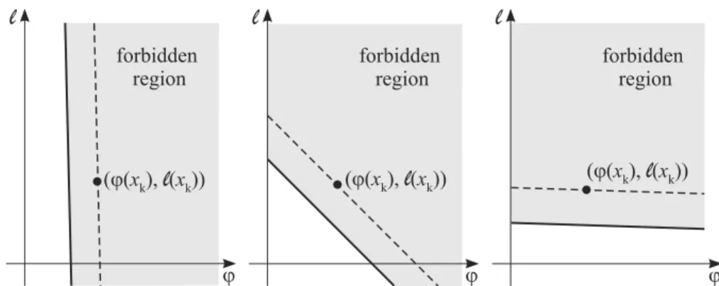
The penalty parameter θ plays a crucial role in the acceptance of the step. For a augmented Lagrangian of the form (2),(θ −1)/θ can be viewed as the slope of the line that defines theforbidden regionin the(ϕ, ℓ)-plane, that is, the semi-space that contains all of the points that are not acceptable at the current iteration. This is illustrated in Figure 1, where the forbidden region is highlighted for different values ofθ.
Figure 1 – Three merit functions on the(ϕ, ℓ)-plane, showing the influence of the penalty
parameterθ. On the left,θ=1/50. In the middle,θ =1/2. On the right,θ =49/50.
Merit functions have been criticized for many reasons. First, it is not so easy to choose an initial value forθ, sinceℓ(x, λ)andϕ(x)usually have very differ-ent meanings and units. Besides, it is necessary to decreaseθ as the algorithm progresses to force it to find a feasible solution. If the initial penalty parameter used is near to 1 andθ is decreased slowly, the algorithm may take too many iterations to reach a feasible point. On the other hand, starting from a small θ or decreasing this factor too quickly may force iterates to stay almost feasible, shortening the steps even when we are far from the optimal solution.
inducing some zigzagging in many cases. This undesired behavior can be con-trolled if an efficient choice of the non-monotonicity parameter is adopted, but this choice is also very problem dependent, so the criticism of the method still applies.
1.2 The filter method
To overcome some of the difficulties inherent to merit functions, Fletcher and Leyffer [8] introduced the idea of using a filter. Instead of combining infeasibility and optimality in one single function, the filter method borrows the idea of nondominance from multi-criteria optimization theory. Thus, a trial point is refused only if it is dominated by some other point, generated in a previous iteration.
This approach was promptly followed by many authors, mainly in conjunction with SLP (sequential linear programming), SQP and interior-point type methods (see, for instance, [1, 5, 6, 7, 9, 11, 12, 15, 16, 17, 22, 23, 24, 25]).
The SQP-filter algorithm presented in [6] illustrates how this nondominance criterion works. In this method, the objective function f is used to measure optimality, while infeasibility is measured by
φ(x)=max
0, max
i=1,···,m|Ci(x)|, i=max1,···,n[xi −ui], i=max1,···,n[li −xi]
.
Functionφ (x)differs fromϕ(x)in the norm used. Besides, the violation of the bound constraints is also taken in account here, since the filter method do not require the iterates to satisfy these constraints.
For each approximate solution x, we can plot a point (φ (x), f(x)) in the (φ, f)-plane, just as we did with (ϕ(x), ℓ(x)) in Figure 1. A third equivalent plane will be introduced in next section, as the algorithm presented in this paper works with(ϕ, f)pairs.
LetF be a set of previously generated pairs in the form (φj, fj). An iterate
xkis accepted by the filter whenever it satisfies
φ(xk) < (1−γ )φj or f(xk) < fj −γ φ(xk) for all (φj, fj)∈F, (6)
One advantage of this type of Pareto dominance criterion is that it does no require the redefinition of a penalty parameter at each iteration. However, to avoid the acceptance of iterates that are too close to the points inF, it was necessary to add to the last inequality of (6) a term that depends on the infeasibility, giving a merit function flavor to this specific filter.
The main disadvantage of the SQP-filter based on (6) is that this acceptance criterion is too tolerant. In fact, requiring only the infeasibilityorthe optimality to be improved makes possible the acceptance of points that are only marginally less infeasible but have a large increase in f(x)over the current iterate, or vice-versa.
Even though, the SQP-filter method can give us some good hints on how to improve the algorithms based on merit functions.
The first hint is that the same merit function that is reliable for points in the (ϕ,f)-plane that are near to(ϕ(xk), f(xk))may be not so useful when the step
is large, so the trial point is far from the current iterate. As illustrated in Figure 1, for values ofθ near to 1, the acceptance criterion based on a merit function cuts off a significant portion of the feasible region, including, in many cases, the optimal solution of the problem.
The second good idea behind the SQP-filter method is that a restoration step should be used sometimes. The objective of a restoration is to obtain a point that is less infeasible than the current one and is also acceptable for the filter. In [6, sec. 15.5], a restoration step is computed when the trust region quadratic subproblem is incompatible (i.e. has an empty feasible set). In our method, this strategy will be used whenever staying away from feasibility seems not worthwhile. In other words, infeasible iterates are welcome only if they generate large reductions of the objective function. If the decrease in f is small and the current point is very infeasible, it is better to move off and find a more feasible point.
1.3 Motivation and structure of the paper
The objective of this paper is to present an algorithm that takes advantages from both the merit function and the filter ideas. The algorithm introduced here is a merit function SQP method, in the sense that it still combines feasibility and optimality in one single function and it still uses penalty parameters. However, not one but several penalty parameters are defined per iteration, each one re-lated to a portion of the(f, ϕ)-space. These parameters are also automatically computed from some(f, ϕ)-pairs collected at previous iterations, so no update scheme need to be defined forθ.
This paper is organized as follows. In the next section, we present the piece-wise linear function we use to accept or reject points. Section 3 introduces the proposed algorithm. In section 4, we prove that the algorithm is well defined. Sections 5 and 6 contain the main convergence results. Finally, in section 7 some conclusions are presented, along with lines for future work.
Through the paper, we will omit some (or even all) of the arguments of a function, if this does not lead to confusion. Therefore, sometimes Q(H,x,s) will be expressed asQ(s), for example, if there is no ambiguity onH andx.
2 A merit function that uses several penalty parameters per iteration
As we have seen, a merit function deals with two different concepts: the infea-sibility and the optimality of the current point.
In this paper, we will introduce a new merit function that uses information collected at previous iterations to accept new points. Since we compare points generated at different stages of the algorithm, this function cannot be based on the augmented Lagrangian, like in [10], as it would depend on the Lagrange multiplier estimates used and, obviously, these estimates change from one iter-ation to another. Therefore, we decided to adopt the so calledsmoothℓ2merit function, defined as:
ψ(x, θ )=θf(x)+(1−θ )ϕ(x). (7)
The actual reduction of theℓ2merit function will be given by Ar ed(x,s, θ )=θA
opt
where
Aoptr ed(x,s)= f(x)− f(x+s) and Ar edf sb(x,s)=ϕ(x)−ϕ(x+s).
Similarly, the predicted reduction of the merit function will be defined as in (3), replacing (5) by
Pr edopt(H,x,s)=Q(H,x,0)−Q(H,x,s),
where
Q(H,x,s)= 1 2s
T
H s+ ∇f(x)Ts+ f(x). (8)
Generally, for a trial point to be accepted, it is necessary that the actual reduc-tion of the merit funcreduc-tion satisfies
Ar ed(x,s, θ )≥ηPr ed(H,x,s, θ ),
whereη∈(0,1)is a given parameter.
However, this scheme based on a linear merit function is usually unreliable for trial points that are far from the current iterate. Therefore, we suggest the use of a piecewise linear function to accept or reject new points, which correspond to use several merit functions per iteration.
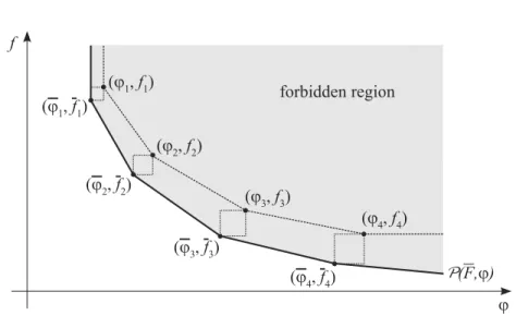
In order to define the new merit function, letFbe a set ofppoints(ϕi, fi)in the
(ϕ,f)-plane. Suppose that these pairs are ordered so thatϕ1< ϕ2<· · ·< ϕp. Suppose also that each point (ϕi, fi) in F is below the line segment joining
(ϕi−1, fi−1)and(ϕi+1, fi+1), fori = 2, . . . ,p−1. Thus the piecewise linear function that passes through all of the points inF is convex.
For each point(ϕi, fi)in F, define another point(ϕi, fi)by moving a little
towards the southwest (a precise definition ofϕi and fi is given in (10) and (11) below). LetF be the set of points(ϕi, fi). The convex piecewise linear
function that connects the points inF is defined by
P(F, ϕ)=
∞, if ϕ < ϕ1;
(fi− fi−1) (ϕi−ϕi−1)ϕ+
(fi−1ϕi− fiϕi−1)
Figure 2 – The setFand the piecewise linear functionP(F, ϕ).
whereγs is a small positive constant, such as 10−4.
This new function, illustrated in Figure 2, is formed by p+1 line segments that can be viewed as merit functions in the form (7). Thei-th of these functions is defined by the penalty parameter
θi =
0, ifi =0; ϕi+1−ϕi
fi−fi+1+ϕi+1−ϕi
, ifi < p;
1/(1+γs), ifi = p.
(9)
and a particular choice ofηthat will be defined below.
The region between the piecewise linear function that passes through the points inFand the function defined byFacts as a margin that prevents the acceptance of iterates that are not “sufficiently” better than the pairs inF.
At each iteration k, Fk is generated defining, for each point (ϕi, fi) ∈ Fk,
another point(ϕi, fi)such that,
ϕi =min ϕi −γcP f sb
r ed (xk,sc), (1−γf)ϕi
, (10)
and
fi =min fi −γfP opt
r ed(Hk,xk,sc), fi−(ϕi−ϕi)
, (11)
for some 0< γf < γc<1. Reasonable values for these constants areγf =10−4
Our algorithm starts with F0= ∅. At the beginning of an iteration, sayk, we define the temporary setFk as
Fk =Fk
(f(xk), ϕ(xk))
.
As it will become clear in the next section, depending on the behavior of the algorithm, the pair (f(xk), ϕ(xk)) may be permanently added to Fk+1 at the end of the iteration. In this case, each pair(f(xi), ϕ(xi))that is not below the
line segment that joins(f(xi−1), ϕ(xi−1))to(f(xi+1), ϕ(xi+1))is removed from
Fk+1, to keep theP(F, ϕ)function convex.
A new iteratex+ = xk +sc is rejected if f(xk +sc)is above the
piecewise-linear functionP(Fk, ϕ(xk+sc))or if we predict a good reduction for the merit
function, but the real reduction is deceiving (in the sense that (14) occurs). To express the first of these conditions in the SQP jargon, we say thatx+is not accepted if
Ar ed(xk,sc, θk)≤ηPr ed(Hk,xk,sc, θk), (12)
where
θk =
θ0, if ϕ(x+) < ϕ1; θi, if ϕi ≤ϕ(x+) < ϕi+1; θp, if ϕ(x+)≥ϕp.
(13)
The η parameter is used in (12) to define the region between Fk and Fk.
However, a formula forηcannot be written explicitly since we do not know in advance which of the terms in (10) and (11) will be used to defineϕi and fi.
Fortunately, this formula will only be used in the proof of Lemma 15 and, in this case, a simple expression is known.
Some agreement between the model function and the objective function of (1) is an usual second requirement for accepting the step in filter methods. In the SQP-filter method presented in [6], for example, this extra condition is used wheneverPr edopt is sufficiently greater than a small fraction of the infeasibility at xk. In this case,sc is only accepted if A
opt r ed/P
opt
r ed > γg is satisfied. Most filter
The combination of infeasibility and optimality into a single merit function allow us to adopt a less stringent condition, rejectingx+only if
Pr edopt(Hk,xk,sc)≥κϕ(xk) and θ
sup
k < γm, (14)
where
θsupk =sup θ ∈R| Ar ed(xk,sc, θ )≥γgPr ed(Hk,xk,sc, θ )
, (15)
κ >0,γm ∈(0,1)andγg∈(0,1).
In words, (14) states that when we predict a good reduction for the optimality part of the merit function, the step is only accepted if there exists a penalty parameterθsupk ∈ [γm,1]such thatAr ed/Pr ed ≥γg.
This condition seems to be somewhat inelegant, since one should expect that all of the iterates that do not belong to the forbidden region shown in Figure 2 are to be accepted. However, if we choose a smallγm, say 10−4, (14) becomes
less stringent than (12) in most cases, so it is seldom used. In fact, we generally haveθ0(≡0) < γm < θ1, so this condition only applies whenxk is the leftmost
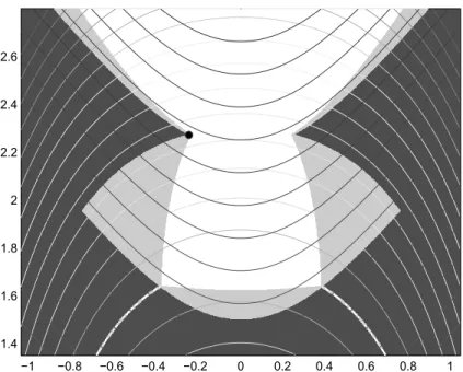
point inF. And even in this case, the forbidden region is only slightly enlarged. Finishing this section, Figure 3 illustrates how the new merit function reduces the region of acceptable points in comparison with the filter. The comparison was made for problem 7 from the Hock and Schittkowski test collection [18]. In the figure, the current iterate,xk =(−0.25,2.27)is shown as a black dot. The points
in the(ϕ,f)-space used to define theF set were(0.01,−1.5), (2.28,−2.21) and(20,−2.7). The forbidden region for the filter method, as defined in (6), is given in dark gray. The points that are acceptable for the filter but not for the new merit function are shown in light gray. The white region contains the points that are acceptable by both criteria. The contour lines of f(x)=log(1+x12)−x2 are concave up, while concave down contour lines are related to the constraint C(x) = (1+x12)2+x2
2 −4. The white concave down narrow region in the bottom of the graph corresponds to points that are almost feasible, i.e., points that satisfyϕ(x) <0.01.
3 An SQP algorithm
−1 −0.8 −0.6 −0.4 −0.2 0 0.2 0.4 0.6 0.8 1 1.4
1.6 1.8 2 2.2 2.4 2.6
Figure 3 – The difference between forbidden regions. Light gray points are accepted by
the filter but not by the new merit function.
of an iteratexk, by a quadratic programming (QP) problem.
In our case, this QP problem has the form
minimize Q(Hk,xk,s)
subject to A(xk)s+C(xk)=0 (16)
l≤xk+s ≤u
s∞≤,
whereQ(H,x,s)is defined by (8),xkis supposed to belong to
= x ∈Rn|l≤ x ≤u
andHkis an approximation of the Hessian of the Lagrangian atxk. It should be
noticed that Hk does not need to be positive definite, so this problem must be
We will use the termϕ-stationaryto say that a pointxˆ satisfies the first order optimality conditions of
minimize ϕ(x) (17)
subject to x ∈.
Unfortunately, ifxk is notϕ-stationary, the constraints of (16) may be
incon-sistent, so this problem may not have a solution. Some algorithms, such as the SQP-filter method presented in [6], include arestorationstep, called to find a new point that makes (16) compatible. Another common practice to overcome this difficulty is to directly divide the stepsc into two components. The first of
these components, callednormal step, or simplysn, is obtained as the solution
of the feasibility problem
reduce M(xk,s)
subject to l≤xk+s ≤u (18)
s∞≤βd.
whereβd ∈(0,1]is a given constant. If M(xk,sn) =0, thenxk can be
substi-tuted by xk +sn in (16) to make this problem feasible, so it can be solved by
any QP algorithm. Otherwise, the second component ofsc, called thetangential
step, orst, is computed soQis reduced but the predicted reduction of the
infea-sibility obtained so far is retained. In other words,scis the solution of the (now
consistent) problem
reduce Q(Hk,xk,s)
subject to A(xk)s = A(xk)sn (19)
l≤ xk+s ≤u
s∞≤.
Usually, βd is set to some value around 0.8 so the trust region is enlarged
from (18) to (19). This is done to preventsnfrom being the the only solution of
(19) when this point is in the border of the trust region of (18). To insure a sufficient decrease ofM, a Cauchy point,sdec
n , is computed. This
the orthogonal projection ofxk− ∇ϕ(xk)on. The solution of (18) is required
to keep at least ninety percent of the reduction obtained bysndec. A similar procedure is adopted for (19). In this case,sdec
t , the Cauchy point,
is obtained from a descent direction for f(x) on the tangent space, given by Px(−∇Q(sn)), the orthogonal projection of−∇Q(sn)on the set
T = y ∈N(A(xk))|(xk+sn+y)∈
.
Again, the decrease on Q obtained by the solution of (19) must not be less than a fixed percentage of the reduction supplied by the Cauchy point.
Besides using this two-step scheme, the algorithm presented here also performs a restoration whenever the step becomes too small and the current point is very infeasible. Although this feasibility reinforcement seems to be unnecessary, the restoration plays a very important role in accelerating the method and keeping the trust region radius sufficiently large.
This role is better explained by an example. Going back to Figure 2, let’s suppose that the current iteratexkis represented by(ϕ4, f4)and that the optimal point has a function value greater than f1. In this case, unless the trust region radius is sufficiently large and our quadratic model is really good (so the algorithm can jump over a large portion of the forbidden region), it will be necessary to perform a considerable number of short-step iterations to traverse from the southeast to the northwest part of the figure. To shorten the path between the current point and the desired solution, it is necessary to focus only on reducing the infeasibility, and this is exactly what the restoration step does.
One may notice that the use of a standard filter is not useful for circumventing this difficulty. In fact, the problem is aggravated in the presence of (almost) right angles in the frontier of the forbidden region. To see why this happens, let’s suppose now that the restoration is used only to ensure that problem (16) is compatible and thatxk is in the vicinity of an almost horizontal segment of the
filter envelope. In this case, to escape from this region, it may be necessary to severely reduce the trust region radius before (16) becomes inconsistent, so the restoration is called.
P(F). An initial pointx0∈ , an initial trust-region radius0≥ minand an initial symmetric matrixH0need also to be given.
Algorithm 1. A new SQP algorithm
1. WHILE the stopping criteria are not satisfied 1.1. Fk←Fk{(f(xk), ϕ(xk))};
1.2. IFC(xk) =0 (xk is feasible),
1.2.1. sn←0;
1.3. ELSE
1.3.1. Computedn (a descent direction forϕ(x)):
dn←Pω(xk−γn∇ϕ(xk))−xk;
1.3.2. Determinesdec
n (the decrease step forϕ(x)), the solution of
minimize M(xk,s)
subject to l≤xk+s ≤u
s∞≤βdk
s =tdn, t≥0;
1.3.3. Computesn(the normal step) such that
l ≤xk+sn≤u,
sn∞≤βdk, and
M(xk,0)−M(xk,sn)≥βm[M(xk,0)−M(xk,sndec)];
1.4. Computedt (a descent direction for f(x)on the tangent space):
dt← Px(−γt∇Q(sn));
1.5. Determinestdec(the decrease step for f(x)), the solution of minimize Q(s)
subject to l ≤xk+s ≤u
s∞≤k
s =sn+tdt, t ≥0;
1.6. Compute a trial stepscsuch that
A(xk)sc= A(xk)sn,
l ≤xk+sc≤u,
sc∞≤k, and
1.7. IF (f(xk+sc)≥P(Fk, ϕ(xk+sc))) OR
(Pr edopt(Hk,xk,sc)≥κϕ(xk)ANDθ
sup
k < γm),
1.7.1. k←αRmin{k,sc∞}; (reduce)
1.8. ELSE 1.8.1. ρk←A
opt
r ed(xk,sc)/P opt
r ed(Hk,xk,sc);
1.8.2. IF Pr edopt(Hk,xk,sc) < κϕ(xk)ORρk < γr,
1.8.2.1. Fk+1←Fk; (include(f(xk), ϕ(xk))in F)
1.8.3. ELSE Fk+1←Fk;
1.8.4. Accept the trial point:
xk+1←xk+sc;
˜
ρk ←Ar ed(xk,sc, θ
sup
k )/Pr ed(Hk,xk,sc, θ
sup
k );
k+1←
max{αRmin{k,sc∞}, min}, if ρ˜k < γg,
max{αAk, min}, if ρ˜k ≥η;
Determine Hk+1; k←k+1;
1.9. IFk < r est ANDϕ(xk) > ǫh2k,
1.9.1. Compute a restoration stepsr so that
(ϕ(xk+sr) < ǫh2k AND f(xk +sr) <P(Fk, ϕ(xk+sr)))
OR xk+sr isϕ-stationary but infeasible;
1.9.2. Fk+1←Fk; (include(f(xk), ϕ(xk))inF)
1.9.3. Accept the new point:
xk+1←xk+sr;
k+1← max{βrr est, min};
Determine Hk+1; k←k+1;
The constants used here must satisfy 0 < βd ≤ 1, 0< βm <1, 0< βq <1,
κ > 0, 0 < γr < γg < η < 1, γn > 0, γt > 0, 0 < min < r est,
0< αR <1,αA ≥1,ǫh >0 andβr >0. Parametersκ,γn,γt,min,r est,ǫh
andβr are problem dependent and must be chosen according with some measure
of problem data. Reasonable values for the remaining parameters might be βd =0.8,βm =0.9,βq =0.9,γr =0.01,γg =0.05,η=0.9,αR =0.25 and
αA =2.5. The constantηshould not be confused with the parameterηdefined
Algorithm 1 seems to be somewhat inefficient, since it requires the solution of several quadratic programming problems per iteration. However, as it will become clear at section 7, only steps 1.3.3 and 1.6 usually require the solution of a quadratic problem. Besides, we do not need to solve these problems exactly, so the algorithm is competitive with modern nonlinear programming codes.
The restoration step is called whenever the trust region radius becomes too small compared toϕ(xk). In this case, we need to find a point that is less infeasible
thanxk and that is also acceptable for the piecewise linear merit function. To
ensure that such a point can always be obtained, it would be necessary to use an algorithm for global minimization. Of course, this alternative is unaffordable, so the restoration is computed in practice by an algorithm for solving the box constrained problem (17). The only drawback of this approach is that we cannot guarantee that a stationary but infeasible point would not be reached. Therefore, we say that the main algorithm fails if this happens.
If xk is feasible, then the condition P opt
r ed < κϕ(xk) is never satisfied, since
Pr edopt is always greater or equal to zero. Besides, the condition Ar edopt < γrP opt r ed
is also never satisfied whenxkis feasible and f(xk+sc) <P(Fk, ϕ(xk+sc)).
Therefore, all of the points in Fk are infeasible, although Fk may contain a
feasible point. This result is very important for two reasons. First, it prevents the optimal solution of problem 1 from being refused by the algorithm. Moreover, it also assures that the algorithm is well defined, as stated in the next section.
4 The algorithm is well defined
An iteration of algorithm 1 ends only when a new pointxk+sis below the
piece-wise linear functionP(Fk, ϕ(xk+s)), besides satisfying some other conditions
stated at steps 1.7 or 1.9.1. While such a point is not found, the trust region ra-dius is reduced and the iteration is repeated. It is not obvious that an acceptable point will be obtained, as we may generate a sequence of points that are always rejected by the algorithm. In this section, we prove that the algorithm is well defined, i.e. a new iteratexk+1can always be obtained unless the algorithm stops by finding aϕ-stationary but infeasible point or a feasible but not regular point.1
In the following lemma, we consider the case wherexk is infeasible.
Lemma 1. Ifxkis notϕ-stationary, then after a finite number of repetitions of
steps1.1to1.9, a new iteratexk+1is obtained by the algorithm.
Proof. At each iterationk, if f(xk +sc) <P(Fk, ϕ(xk+sc))and one of the
conditions
Pr edopt(Hk,xk,sc)≤κϕ(xk) or Ar ed(xk,sc, θ
sup
k )≥γgPr ed(Hk,xk,sc, θ
sup
k )
(for some θksup ≥ γm) is satisfied, then xk +sc is accepted and we move to
iterationk+1. Otherwise,kis reduced and after some unfruitful steps,k <
r est andϕ(xk) > ǫh2k, so a restoration is called.
Suppose that aϕ-stationary but infeasible point is never reached (otherwise the algorithm fails). As the restoration generates a sequence of steps{sj}
con-verging to feasibility, and sinceFkdoes not include feasible points (becausexk
is infeasible and no feasible point is included inFk), there must exist an iterate
xk+sr that satisfiesϕ(xk+sr) <min{ϕ1, ǫh2k}, so we can proceed to the next
iteration.
Now, in order to prove that the algorithm is also well defined when xk is
feasible, we need to make the following assumptions.
A1. f(x)andCi(x)are twice-continuously differentiable functions ofx.
A2. The sequence of Hessian approximations{Hk}is bounded.
As a consequence of A1 and A2, the difference between the actual and the predicted reduction of the merit function is proportional to2, so the step is accepted for a sufficiently small trust region radius, as stated in the following lemma.
Lemma 2. Suppose that A1 and A2hold and thatxk is feasible and regular
for problem1but the KKT conditions do not hold. Then, after a finite number of trust region reductions, the algorithm finds a new pointxk+sc that satisfies
f(xk+sc) <P(Fk, ϕ(xk+sc))andAr ed(xk,sc, θ
sup
k )≥γgPr ed(Hk,xk,sc, θ
sup
k )
Proof. Since xk is feasible, sn = 0. Supposing that xk is regular and
non-stationary, there must exist a vectordt =0 satisfying
l≤xk+dt ≤u, A(xk)dt =0, and dtT∇f(xk) <0.
Let us define, for all >0,
p()=t()dt,
where
t()=max{t >0| [xk,xk+tdt] ⊂, and tdt∞≤}. (20)
Clearly,x+dt ∈, so we have thatt()dt∞=whenever≤ dt∞.
Define, in this case,
c = −1 2d
T
t ∇f(xk)/dt∞= −
1 2d
T
t ∇Q(0)/dt∞>0.
Since Q(sdec
t ) ≤ Q(p()), by elementary properties of one-dimensional
quadratics, there exists1∈(0,dt∞]such that, for all∈(0, 1),
Q(0)−Q(stdec)≥ −1 2d
T
t ∇Q(0)t()= −
1 2
dT t ∇Q(0)
dt∞
=c.
Moreover, since xk is feasible and Asn = 0, we have that M(xk,0) =
M(xk,sc)=0, so
Pr edf sb(xk,sc) = 0, and
Pr edopt(Hk,xk,sc()) = Q(0)−Q(sc())
≥ βq
Q(0)−Q(stdec)≥βqc.
(21)
Oncexk is feasible,(ϕ(xk), f(xk))is the first pair inFk. Thus, there exists
2 ∈ (0, 1]such that, for < 2, we need to consider only the portion of
P(Fk, ϕ)defined on the interval[0, ϕ2]. This linear function may be rewritten so the condition
f(xk +sc) <P(Fk, ϕ(xk+sc))
is equivalent to
where,
Pr ed(Hk,xk,sc(), θ1)=θ1P
opt
r ed(Hk,xk,sc())≥βqcθ1, (23)
Ar ed(xk,sc(), θ1)=θ1
f(xk)− f(xk+sc())
+(1−θ1)ϕ(xk+sc())
andθ1>0 is given by (9).
Now, by A1, A2 and the definition of Pr ed, we have
Ar ed(xk,sc, θ )= Pr ed(Hk,sk,sc, θ )+c1sc2. (24)
So, using (23) and (24) we deduce that
Ar ed()
Pr ed() −
1 ≤
|c1|
βqcθ1
. (25)
Thus, for <min (1−η1)βqcθ1/|c1|, 2
=3, the inequality (22) nec-essarily takes place.
Now, using the fact thatθsupk =1 forxkfeasible and replacingθ1by 1 in (25), we can conclude that, for
<min (1−γg)βqc/|c1|, 3
=4, (26)
the condition Ar ed(xk,sc(), θ
sup
k ) ≥ γgPr ed(Hk,xk,sc(), θ
sup
k )is also
satis-fied and the step is accepted.
5 The algorithm converges to a feasible point
As mentioned in the last section, our algorithm can stop if aϕ-stationary but infeasible point is found. Naturally, this unexpected behavior of the algorithm makes somewhat pretentious the title of this section.
Formally, what we will prove is that, supposing that aϕ-stationary but infea-sible point is never reached and that the restoration always succeeds, an infinite sequence of iterates converges to feasibility.
In the proofs of the lemmas presented here, we will suppose that A1 and the following assumption are satisfied.
This requirement is easy to fulfill, as we usually can define finite lower and upper limits for the variables. Besides, as mentioned in [6, p. 730], assumptions A1 and A3 together ensure that, for allk,
fmin ≤ f(xk)≤ fmax and 0≤ϕ(xk)≤ϕmax
for some constants fmin, fmax andϕmax > 0. Our analysis will be based on the fact that the rectangle A0 = [0, ϕmax
] × [fmin, fmax
]is covered by a finite number of rectangles with area greater than a small constant. Therefore, each time we expand the forbidden region (see fig. 2) by adding to it a small rectangle, we drive the iterates towards feasibility.
Let us start investigating what happens toϕ(x)when an infinite sequence of iterates is added toF, following the skeleton of Lemma 15.5.2 of [6].
Lemma 3. Suppose that A1and A3hold and that {ki}is any infinite
subse-quence at which the iteratexki is added toF. Then
lim
i→∞ϕ(xki)=0.
Proof. Let us suppose, for the purpose of obtaining a contradiction, that there exists an infinite subsequence{kj} ⊆ {ki}for which
ϕ(xkj)≥ǫ, (27)
whereǫ >0.
At iterationkj, the(ϕ, f)-pair associate withxkj is included inFat positionm,
which means thatϕm−1≤ϕk
j(≡ϕm)≤ ϕm+1and fm−1≥ fkj(≡ fm)≥ fm+1.
Thus, as long as the pair(ϕkj, fkj)remains inF, no other(ϕ, f)-pair is accepted
within the rectangle
rm = (ϕ,f)|ϕm ≤ϕ ≤ϕm, fm ≤ f ≤ fm
.
Notice that, by (10), (11) and (27), the area of this rectangle is, at least,
(ϕm −ϕm)(fm− fm)≥(ϕm−ϕm)
2
≥(γfϕkj)
2
≥γ2fǫ2.
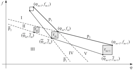
Assume now that (ϕk
j, fkj) is excluded from F by another pair (ϕkl, fkl),
that(ϕk
l, fkl)cannot fall in regions I and V since, in this case,(ϕkj, fkj)will not
be excluded from F. It can be easily verified that the worst case occurs when (ϕkl, fkl)lies on p1(ϕ)or p2(ϕ).
Suppose(ϕk
l, fkl)lies onp2(ϕ), as depicted in Fig. 4. In this case, the rectangle
rm will be entirely above p2, the line that connects(ϕkl, fkl)to(ϕm+1, fm+1).
Since p2will be included in the new piecewise linear function P(F), no point withinrm can ever be reached by a new iterate.
The same idea can be applied in the case(ϕkl, fkl)lies on p1(ϕ). Therefore,
once(ϕkj, fkj)is included in F,rm will always be aboveP(F). Since the area
of this rectangle is at leastγf2ǫ2and the set A0is completely covered by at most Surf(A0)/[γ2fǫ2]of such rectangles, it is impossible for an infinite subsequence of{ki}to satisfy (27), and the conclusion follows.
Figure 4 – Adding a new iterate that excludes(ϕkj,fkj)fromF.
Finally, we are going to consider the case where no point is added to Fk fork
sufficiently large.
Lemma 4. Suppose that assumptions A1and A3hold. Suppose also that, for allk >k0,xk is never included in Fk. Then,
lim
Proof. Sincexkis not included inFk, no restorations are made and both
condi-tions stated at step 1.8.2 of algorithm 1 are never satisfied fork >k0. Therefore, we have
f(xk)− f(xk+1)≥γrP opt
r ed ≥γrκϕ(xk) >0, (29)
for allk >k0, which means that the objective function always decrease between infeasible iterations. Since A1 and A3 imply fmin ≤ f(xk) ≤ fmax, we must
have
lim
k→∞ f(xk)− f(xk+1)=0. (30) Then, (28) follows from (29) and (30).
6 The algorithm finds a critical point
Finally, we are able to prove the convergence of the algorithm to a stationary point for (1). In order to do that, we will need to make one additional assumption on the choice of the normal stepsn.
A4. There existκn,kN >0 such that, if{xki}is a subsequence of iterates that
converges to a feasible point, the choice ofsnat step 1.3.3 of algorithm 1
satisfies
sn(xk, k) ≤κnC(xk)2
forki >kN.
This requirement is also easy to fulfill since it only applies when the infeasi-bility is small and, in this case, it is reasonable to suppose that the normal step will also be small.
In the following lemma, derived from Lemma 6.1 of [10], we show that in the neighborhood of a feasible, regular and non-stationary point, the directional derivative of the quadratic model (8) alongdt is bounded away from zero.
Lemma 5. Suppose that A2 and A4hold and that {xki}is an infinite subse-quence that converges to the feasible and regular point x∗ ∈ , which is not stationary for(1). Then there existsk1,c1>0such that
for allx ∈ {xki | k ≥ k1}. Moreover,dt(H,x, )is bounded and bounded away from zero for allx ∈ {xki |k ≥k1}.
Proof. For allx ∈ {xki}, we have that
dt(H,x, )= Px(−γt∇Q(sn(x, )))= Px(−γt[H sn(x, )+ ∇f(x)]).
By the contractive property of the orthogonal projections,
Px(−γt[H sn(x, )+ ∇f(x)])−Px(−γt∇ f(x))2≤γtH2sn(x, )2.
So, by A2 and A4, we have that
dt(H,x, )−Px(−γt∇f(x))2≤γ1C(x) (32)
fork > kN. By the continuity of∇ f(x)and the fact that{xki}converges, we
deduce that
∇f(xki)
T
Px(−γt∇f(xki))− ∇f(xki)
T
dt(Hki,xki, ki)2≤γ2C(xki). (33)
Notice that Px(−γt∇f(xki))is the solution of
minimize −γt∇f(xki)−z
2 2 subject to A(xki)z =0
l≤xki +sn+z ≤u.
Now, definePx∗(−γt∇ f(x∗))as the solution of
minimize −γt∇f(x∗)−z22
subject to A(x∗)z =0 (34) l ≤x∗+z≤u.
Since x∗ is regular but is not a stationary point for (1), it follows thatz = 0 is not a solution for (34). So, Px∗(−γt∇f(x∗)) =0. Moreover, sincez =0 is
feasible for (34), we have that
which implies that∇f(x∗)TP
x∗(−γt∇f(x∗)) <0.
Using the fact that Px(−γt∇f(x))is a continuous function ofx andsnfor all
regularx (see [10]), we can definec2,c3,c4 > 0 andk2 ∈ Nsuch that, for all
x ∈ {xki |k ≥k2}, we have
c2≤ Px(−γt∇f(x)) ≤c3 and ∇f(x)TPx(−γt∇ f(x))≤ −c4. (35)
Now, from (32), (33) and (35), the continuity ofC(x)and the feasibility of x∗, there existsk3≥max{k2,kN}such that, wheneverx ∈ {xki |k≥k3},
c2
2 ≤ dt(H,x, ) ≤2c3 and ∇f(x)
Td
t(H,x, )≤ −
c4 2 .
Therefore, dt(H,x, ) is bounded and bounded away from zero for all
x ∈ {xki |k ≥k3}.
Finally, since dt ∈ N(A(x)), assumptions A2 and A4 hold, and dt is
bounded, we have that, for allx ∈ {xki |k≥k3},
∇Q(sn)Tdt = ∇f(x)Tdt+dtTH sn ≤ −
c4
2 +γ3C(x),
whereγ3 > 0. Then, (31) follows defining c1 = c4/4 and choosing k1 > k3 such thatC(x) ≤c4/(4γ3). Using Lemma 5, we state in the next lemma that, in the neighborhood of a feasible, regular and non-stationary point, the decrease of the quadratic model (8) is proportional to the trust region radius.
Lemma 6. Suppose that A2 and A4hold and that {xki}is an infinite subse-quence that converges to the feasible and regular point x∗ ∈ , which is not
stationary for(1). Then there existsc2,k2>0and1∈(0, min)such that Q(x,sn(x, ))−Q(x,sc))≥c2min{, 1} (36)
for allx ∈ {xki |k ≥k2}.
Proof. See Lemma 6.2 of [10].
Lemma 7. Suppose that A1, A2 and A4 hold and that {xki} is an infinite subsequence that converges to the feasible and regular pointx∗ ∈ , which is not stationary for(1). Then there existsǫ,c3,k3 >0and1∈ (0, min)such that, forki >k3, if
ϕ(xki)≤ǫ
2
, (37)
we have that
Pr edopt(xki,sc)=Q(xki,0)−Q(xki,sc)≥c3min{, 1}. (38)
Proof. By Lemma 6, assumptions A1 and A4 and the convergence of{xki}, we
have that
Q(0)−Q(sc)≥ Q(sn)−Q(sc)−|Q(0)−Q(sn)| ≥c2min{, 1}−γ4C(x) for allx ∈ {xki |k ≥ k2}, wherec2,k2 and1are defined as in Lemma 6 and
γ4 > 0. Therefore, (38) follows if we choosec3 < c2 andk3 ≥ k2 such that ǫ≤α2(c2−c3)2/(2γ2
4), whereα =min{1, 1/}. We next examine what happens ifis bounded away from zero and an infinite subsequence of points is added toF.
Lemma 8. Suppose that A1, A2, A3andA4hold and that{xkj}is an infinite subsequence at whichxkj is added toF. Suppose furthermore that the limit points of this sequence are feasible and regular, that the restoration always terminates successfully and thatkj ≥2, where2is a positive scalar. Then there exists a limit point of this sequence that is a feasible, regular and stationary point for(1).
Proof. From assumption A3, we know that{xkj}has a convergent subsequence,
say{xki}. Let us suppose that the limit point of this subsequence is not stationary
for (1).
From Lemma 3 we know that there existsk5∈Nsuch that, forki >k5,
ϕ(xki) < ǫh
Thus, a restoration is never called for ki > k5. So, the hypothesis that xki
is added to Fki implies that Ar ed(xki,sc, θ
sup
ki ) ≥ γgPr ed(xki,sc, θ
sup
ki ) for some
θksup
i ≥γm, and that one of the inequalities stated at step 1.8.2 of the algorithm is
satisfied at iterationki.
Suppose, for the purpose of obtaining a contradiction, that{xki}converges to
a point that is not stationary for (1). So, from Lemma 3 and (38), there exists k6≥k5such thatϕ(xki) < ǫ
2
ki and
Pr edopt(xki,sc)≥c3min{1, 2},
for allki >k6.
Using Lemma 3 again, we can deduce that there exists k7 ≥ k6 such that ϕ(xki) < (c3/κ)min{1, 2}and the conditionP
opt
r ed < κϕ(xk)is never satisfied
forki >k7.
Therefore,ρk < γr must hold. To show that this is not possible, let us write
the inequality Ar ed(xki,sc, θ
sup
ki )≥γgPr ed(xki,sc, θ
sup
ki ), as
θsupk
i A
opt
r ed(xki,sc)+(1−θ
sup
ki )(ϕ(xki)−ϕ(xki +sc))
≥γgθ
sup
ki P
opt
r ed(xki,sc)+γg(1−θ
sup
ki )P
f sb
r ed(xki,sc).
Using the hypothesis thatρk < γr and the fact thatP f sb
r ed (xki,sc)≥0, we have
θsupk
i γrP
opt
r ed(xki,sc)+(1−θ
sup
ki )(ϕ(xk)−ϕ(xk +sc))≥γgθ
sup
ki P
opt
r ed(xki,sc).
Then, taking k4 > k3 (defined in Lemma 7), we deduce from (38) that, for ki >k4,
(1−θsupk
i )(ϕ(xki)−ϕ(xki +sc))≥(γg−γr)θ
sup
ki c3min{1, 2}.
But, since,γg > γr and limi→∞ϕki =0, we must have
lim
i→∞θ sup
ki =0,
which contradicts the fact thatθsupk
i ≥ γm. Therefore,{xki}must converge to a
stationary point for (1).
Lemma 9. Suppose that A1, A2, A3andA4hold, thatxkis always accepted
butFk remains unchanged fork >k5and thatk ≥3, for some positive3.
Suppose also that the limit points of the infinite sequence{xk}are feasible and
regular. Then there exists a limit point of {xk} that is a feasible, regular and
stationary point of(1).
Proof. Assumption A3 implies that there exists a convergent subsequence
{xki}. If the limit point of this subsequence is not stationary for (1), then from
Lemma 7, we have
Pr edopt ≥c3min{3, 1} (39) for allki >max{k5,k3}. Moreover, sincexki is always accepted and Fk is not
changed, we deduce, from step 1.8.2 of the algorithm, thatρk ≥γr. Therefore,
f(xki)− f(xki +sc)≥γrP
opt
r ed. (40)
From (39) and (40) we conclude that f(xki)− f(xki +sc)≥γrc3min{1, 3}
for allki sufficiently large, which contradicts the compactness assumption A3.
Thus, the limit point of{xki}must be stationary.
In the last part of this section, we will discuss the behavior of the algorithm when→0. We will start showing that the predicted reduction of the quadratic model is sufficiently large whenis small.
Lemma 10. Suppose thatA2andA4hold and that{xki}is an infinite subse-quence that converges to the feasible and regular point x∗ ∈ , which is not stationary for(1). Suppose also thatϕk satisfies(37)and that
<min c3/(κǫ), 1
=5 (41)
forki >k6, wherec3,ǫand1are defined as in Lemma7. ThenPr edopt > κϕ(xki).
Proof. Suppose, for the purpose of obtaining a contradiction, that Pr edopt ≤ κϕ(xk)for someki >k6. Then, from (38), we have
c3min{, 1} ≤ Pr edopt ≤κϕ(xki)≤κǫ
2 ,
The purpose of the next four Lemmas is to prove that there exists a sufficiently small trust region radius so the step is always accepted and is not reduced further at step 1.7.1 of algorithm 1.
The first lemma shows the relation between the predicted reduction of the infeasibility and.
Lemma 11. Suppose that assumption A1 holds and thatxkis notϕ-stationary.
Then there exists6,c4>0such that
Pr edf sb(xk,sc)≥c4k, (42)
ifk ∈(0, 6).
Proof. The proof of this Lemma is based on the same arguments used to obtain (21). However, here we deal with the reduction of the infeasibility, instead of the reduction of the objective function, so some modifications need to be done.
Firstly, we must notice thatdn=0, since we suppose thatxkis notϕ-stationary.
Thus, we can redefine (20) as
t()=max t >0| [xk,xk+tdn] ∈ and tdn ≤βd
.
Now, using the fact that forsufficiently small we havet()dn =βdand
defining
c= −1 2d
T
n∇ϕ(xk)/dn>0,
there must exist6∈(0,dn]such that
M(0)−M(t())≥ −1 2d
T
n∇ϕ(xk)t()=cdnt()=βdc
for all∈(0, 6). Therefore, for the normal stepsncomputed at step 1.3.3 of
algorithm 1, we have
M(0)−M(sn)≥βdβmck.
But, since A(xk)sc = A(xk)sn, we deduce from (4) that
Pr edf sb(xk,sc)≥βdβmck
In order to prove thatxk+scwill be accepted, we need to consider howϕand
f are computed. Let us begin using the previous lemma to show that, for a small ,ϕi, defined in (10), will depend on the predicted reduction of the infeasibility.
Lemma 12. Suppose thatA1holds and thatxkis notϕ-stationary. Then there
exists7>0such that γcP
f sb
r ed(xk,sc) > γfϕ(xk),
ifϕ(xk) < ǫh2kandk ∈(0, 7).
Proof. Lemma 11 ensures that γc
γf
Pr edf sb(xk,sc)≥
γc
γf
c4k >0.
Defining7 =min γcc4/(γfǫh), 6
, where6is given in Lemma 11, we have that
γc
γf
Pr edf sb(xk,sc)≥ǫh7 > ǫh2≥ϕ(xk),
for all∈(0, 7), so the desired result follows. Using Lemma 11 again, we can also show that f, defined in (11), will depend onPr edopt ifis sufficiently small.
Lemma 13. Suppose that A1, A2and A4hold, that {xki} is an infinite sub-sequence that converges to the feasible and regular pointx∗ ∈, which is not stationary for(1), and thatϕk is given by(10). Then there exists8 >0such that
γfP opt
r ed(Hk,xk,sc)≥(ϕ(xk)−ϕk),
ifϕ(xk) <min{ǫh, ǫ}k2andk ∈(0, 8), whereǫis defined as in Lemma7.
Proof. From Lemma 7 we deduce that, ifk ∈(0, 1], then γfP
opt
r ed(Hk,xk,sc)≥γfc3k.
Now, defining8=min γfc3/ǫh, 1
, we have
γfP opt
r ed(Hk,xk,sc)≥ǫh8≥ǫh2k ≥ϕ(xk)≥(ϕ(xk)−ϕk)
Let us prove now that, for a infeasiblex, the ratio between the actual and the predicted reduction of the merit function is sufficiently large ifis small, not matter how the penalty parameterθ is chosen.
Lemma 14. Suppose that A1, A2andA4hold, thatθ ∈ [0,1]andγ ∈(0,1)
are given parameters and that{xki}is an infinite subsequence that converges to the feasible and regular pointx∗ ∈, which is not stationary for(1). Then there exists9>0such that, forki sufficiently large,
Ar ed(xki,sc, θ )≥γPr ed(Hki,xki,sc, θ )
for allki ∈(0, 9), ifxki is infeasible.
Proof. Since limi→∞ϕ(xki)=0 and, at the beginning of iterationk, the trust
region radius satisfies ki ≥ min, there must existk7 ≥ k3(defined in
Lem-ma 7) such that, forki > k7, the conditionϕ(xki) ≤ ǫ
2
ki is satisfied, so (38)
holds. Besides, since xki is infeasible, (42) also holds if we take 9 ≤ 6
(defined in Lemma 11). Therefore, from the definition of Pr ed, we have that
Pr ed(Hki,xki,sc, θ )≥θc3min{ki, 1} +(1−θ )c4ki.
where1,c3andc4are defined as in Lemmas 7 and Lemma 11. For anyθ ∈ [0,1], the above inequality implies that
Pr ed(Hki,xki,sc, θ )≥min{ki, 1}min{c3,c4}>0.
But, from A1 and A4, we also have that
|Ar ed(ki)−Pr ed(ki)| ≤c5
2
ki.
for somec5>0. From the last two inequalities, we deduce that, forki ≤1,
|Ar ed(ki)−Pr ed(ki)|
Pr ed(ki)
=
Ar ed(ki)
Pr ed(ki)
−1
≤
c5
min{c3,c4}k. (43)
Therefore, defining9 = min{(1−γ )min{c3,c4}/c5, 1, 6}, we obtain the
required result.
Lemma 15. Suppose thatA1,A2, A3andA4hold. Suppose also that the limit points of the infinite sequence{xk}are feasible and regular and thatlimk→∞k
=0. Then there exists a limit point of{xk}that is a stationary point of(1).
Proof. Assumption A3 implies that there exists a convergent subsequence{xki}.
Let us suppose, for the purpose of obtaining a contradiction, that the limit point of this subsequence is not stationary for (1).
Now, we need to consider separately two mutually exclusive situations. First, let us suppose thatxki is feasible. In this case, Lemma 2 assures that, for < 4
(defined in (26)), the step is accepted and the trust region radius need not to be reduced further.
On the other hand, ifxki is notϕ-stationary, Lemmas 12 and 13 assure that, for
ki ≤min{7, 8} =10, we haveP
f sb
r ed ≥γfϕi/γcandPr edopt ≥(ϕi−ϕi)/γf,
so the parameterηused in (12) is given by
η= (fi−1− fi)γcP
f sb
r ed +(ϕi −ϕi−1)γfP opt r ed
(fi−1− fi)P f sb
r ed +(ϕi−ϕi−1)P
opt r ed
,
whereiis defined in such a manner thatϕi−1 ≤ϕ(x+)≤ϕi. Thus, 0< η <1 and f(xki +sc) >P(Fki, ϕ(xki +sc))is equivalent to (12).
Now, using Lemmas 10 and 14, we can deduce that, forki < 9, the step is
always accepted. Consequently,ki ≥αRmin{4, 9, 10}, which contradicts
the hypothesis that limk→∞k = 0, so we conclude that the limit point of the
subsequence{xki}is a stationary point of (1).
Finally, let us state a theorem that puts together all of the results presented so far.
Theorem 1. Suppose that A1, A2,A3andA4hold and that{xk}is an infinite
sequence generated by Algorithm1. Then either the restoration converges to a ϕ-stationary but infeasible point of (1), or limk→∞ϕ(xk) = 0. Moreover,
if the restoration always succeeds and all of the limit points of {xk} are
regu-lar, there exists a limit point x∗ that is a regular and stationary point for (1). In particular, if all of theϕ-stationary points are feasible and regular, then there exists a subsequence of{xk}that converges to a feasible, regular and stationary
Proof. This result is a direct consequence of Lemmas 3, 4, 8, 9 and 15.
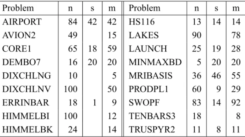
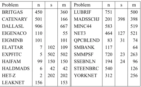
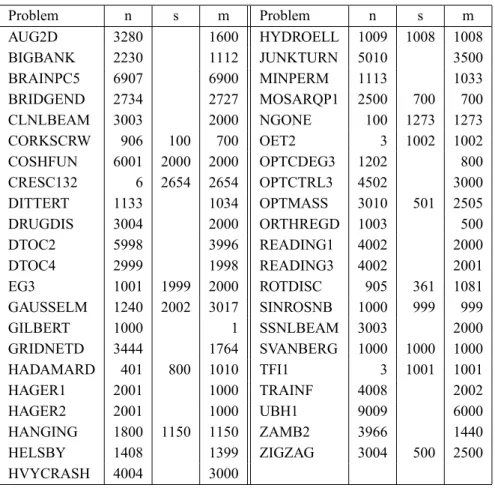
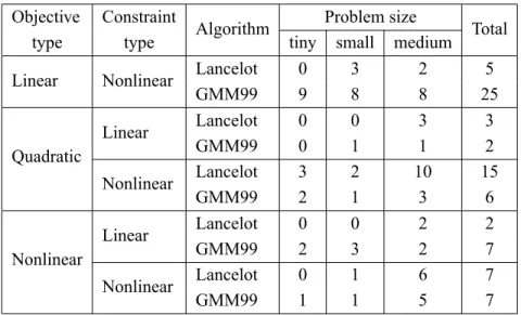
7 Numerical experience
The description of some steps of Algorithm 1 was intentionally left vague to suggest the reader that several alternative implementations are available. In this section, we describe one of such possible implementations and present the numerical results obtained by applying the algorithm to some problems from the CUTEr collection [13].
7.1 Algorithmic details
The computational effort of algorithm 1 may be decomposed into three main parts. The first is related to the reduction of the infeasibility and includes steps 1.3.1 to 1.3.3. The aim of the second part, that comprises steps 1.4 to 1.6, is to improve the objective function. Finally, a restoration is called, at step 1.9.1, if the infeasibility needs to be drastically reduced. Each one of these parts is briefly described below.
Taking a closer look at steps 1.3.1 and 1.3.2, one may notice that vectorsdnand
sdec
n can be easily determined, since the first involves computing a projection on
a box and the second requires only the solution of a one-dimensional problem. The normal step,sn, can be obtained by solving the bound-constrained least
squares problem (18), replacing the wordreduceby minimize. In our experi-ments, the Quacon package [2] was used for this purpose. The computation of snis declared successful when both conditions
M(xk,0)−M(xk,sn)≥βm
M(xk,0)−M(xk,sndec)
and
gp(sn)2≤0.001gp(sndec)2
are satisfied, whereβm = 0.9 andgp is the projected gradient of the quadratic
function minimized. Otherwise, the limit of max{1000,6n}iterations is reached. Vectorscis computed by applying the MINOS 5.4 [19] solver to the quadratic
problem (19), stopping the algorithm when both
gp(sc)∞≤10−6
λ1
√m,1