L. F. de Souza
M. T. de Mendonça
Instituto de Tecnológico de Aeronáutica Pç. Mal. Eduardo Gomes, 50 12228-900 São José dos Campos, SP. Brazil [email protected]M. A. F. de Medeiros
USP - Universidade de São Paulo Escola de Engenharia de São Carlos Av. Trabalhador São Carlense, 400 13566-590 São Carlos, SP. BrazilM. Kloker
Institut für Aerodynamik und GasdynamikUniversität Stuttgart, Germany
Seeding of Görtler Vortices Through a
Suction and Blowing Strip
The resulting wavelength of Görtler vortices in boundary layers over concave surfaces is determined by the upstream history of the flow and by wall disturbances such as roughness, heating/cooling strips or suction and blowing. In isotropic disturbance conditions, the predominant spanwise wavelength corresponds to the strongest growing vortex mode predicted by the linear stability theory. If the disturbance environment is not isotropic, vortices with wavelength different from the one with the highest growth rate may emerge. The present investigation considers the wavelength selection when Görtler vortices are excited by a suction and blowing strip at the wall. The study is based on numerical simulations of the vorticity transport equations derived from the Navier-Stokes equations. They are solved using a compact high-order finite difference technique. The results show that, when the vortices are excited by suction and blowing at the wall, their spanwise wavelength does not necessarily correspond to the imposed wavelength. Curves of streamwise development of the disturbance energy for different harmonics are presented, showing the evolution of the dominant modes. Isolines of streamwise velocity in the spanwise plane are also presented, showing how the higher harmonics distort the characteristic mushroom structures.
Keywords: Görtler vortices, spatial direct numerical simulation, hydrodynamic stability, high order compact finite difference scheme, transition to turbulence
Introduction
Turbulent flows are the most common in practical applications. Nevertheless, there are a large number of situations in which transition to turbulence is of significant importance. That is the case for the flow over low Reynolds number turbine blades and laminar flow airfoils. The understanding of how transition takes place can help in predicting and even controlling transition to turbulence. Over recent years the body of knowledge on laminar flow stability and transition has increased dramatically due to the development of new experimental and numerical techniques as well as due to advances in applied mathematical theories. However, there are many transition scenarios for which a physical explanation is still unknown, and predicting transition location remains a challenge in many engineering applications.1
The study of boundary-layer stability over concave surfaces, started by Görtler (1940), has attracted the attention of several scientists. The centrifugal instability mechanism is responsible for the development of counter-rotating vortices aligned in the streamwise direction, as shown in Fig. 1, known as Görtler Vortices (GV). These vortices pump low momentum fluid away from the wall and high momentum fluid toward the wall forming up-wash and down-wash regions respectively (Fig. 2). The result of this macroscopic redistribution of mass is the development of mushroom type structures with strong inflectional velocity profiles in the normal and spanwise directions. These inflectional velocity profiles are susceptible to high frequency secondary instability further downstream. Reviews on GV with detailed description and theoretical background, have been published by Hall (1990), Floryan (1991) and Saric (1994).
Initially, Görtler vortices have a very weak growth rate and the resulting wavenumber is strongly dependent on the previous history of the flow. Therefore, it is easy to observe a flow structure with a wavelength different from the one corresponding to the fastest growing vortices predicted by Linear Stability Theory (LST). For the same reason, and as shown in the current paper, it may also be difficult to impose a desired wavelength. Several techniques can be
Paper accepted July, 2004. Technical Editor: Aristeu da Silveira Neto.
used to seed GV in the flow field in experimental facilities and numerical simulations. The wavelength can be set by the upstream flow disturbance environment, by surface roughness or by other surface disturbances such as heating and cooling wires or suction and blowing strips. This paper is concerned with the selection of GV wavelength and the way to induce vortices with a desired wavelength using suction and blowing strips.
Figure 1. Görtler vortices over a concave wall.
Analysis of the resulting vortex wavelength is important for boundary layer control through suction and blowing. In principle, GV can be damped if suction and blowing are applied in the vortices up-wash and down-wash regions respectively (Myose and Blackwelder, 1995, Souza, 2001). An estimate of the vortex wavelength would help the control system designer, but the control system itself should not introduce other disturbances with a different wavelength in the flow.
One of the first investigations that addressed the problem of wavelength selection mechanism was due to Bippes (1978). He studied the flow over concave surfaces and presented results for three different upstream conditions: without any disturbance generator, with screens to produce isotropic disturbances and with surface mounted heated wires in order to have controlled disturbances. In all the experiments he found the characteristic counter-rotating vortices. When using screens, Bippes suggests that the selected wavelength follows the maximum amplification curve predicted by LST.
A well documented article presenting experimental results was written by Swearingen and Blackwelder (1987). Their results are frequently used for validation by numerical experimentalists. They did not use any mechanism to generate disturbances and the resulting spanwise pattern was found to depend on the last screen chamber used to control the turbulence level. Myose and Blackwelder (1991) show results where the GV wavelength was modified by varying the amount of tunnel side wall boundary layer removal just upstream of the concave wall test section leading edge. They concluded that when the disturbance field is isotropic the wavenumber corresponding to the strongest amplification is the preferred one.
The importance of the upstream history of the flow was acknowledged by Hall (1982), who proposed that the development of GV is governed by parabolic equations and discarded the normal mode formulation for the early stages of GV development. Further downstream the vortex structures tend to the eigenfunctions predicted by normal modes (Lee and Liu 1992). As a result of the GV parabolic nature, unlike Tollmien-Schlichting waves, it is not possible to define a critical Görtler number Go, where Go is the nondimensional parameter characteristic of boundary layer centrifugal instability. The vortex growth or decay for low values of Go depends on the pre-existing vortical structures in the flow (Hall 1982, Botaro and Luchini, 1999).
Guo and Finlay (1994) studied the wavenumber selection, splitting and merging of Dean and Görtler Vortices. They showed that when the energy level of GV is low, the spatial growth of the vortices is linear. At this stage, vortices with different wavelength can develop at the same time and show no significant interaction with each other. They also found that for large wavenumbers a new pair of vortices with different wavelength is likely to appear, causing a splitting of the original vortices.
Bottaro and Zebib (1997) studied different wall roughness distributions and their influence in the GV formation. They found the preferable wavelength to be near the most amplified LST mode for different disturbance inducers. They also found that triangular riblets are the best GV promoters, but in this case the wavelength is set by the distance between the riblets and not by the mode with the largest amplification rate. They also found that, before the instability mechanism can start to amplify disturbances, there is a linear filtering region called receptivity region.
Luchini and Bottaro (1998) studied the receptivity of GV to free stream disturbances and to wall disturbances. They used adjoint parabolic equations to integrate backward in space and achieve the perturbation sources that give birth to GV. They arrived at the Green’s functions that result in the most amplified GV when scaling external disturbances in a receptivity process. They investigated
external disturbances coming from the free-stream or from the wall, and could identify the disturbance that is most effective in generating GV.
As can be concluded from these investigations, several techniques can be used to ‘seed’ Görtler vortices in experimental facilities and numerical simulations. In this study perturbations are introduced by suction and blowing at the wall in a disturbance strip. The normal velocity component at the wall varies according to a cosine function in the spanwise direction. The results show that there is a receptivity region between the disturbance strip and the region where the disturbances propagate as classic GV. In this receptivity region the perturbations are filtered by the boundary layer and the resulting vortex wavelength is not necessarily the imposed wavelength at the disturbance strip. Tests were made in order to verify the behavior of the flow in the receptivity region and in the subsequent GV dominated region. The study is performed by using Spatial Direct Numerical Simulation (DNS).
In the following sections first the governing equations and the numerical method are presented. Then verification and validation test cases are presented comparing the DNS results with results from other numerical models (Mendonça, 2000, Lee and Liu, 1992, Li and Malik, 1995) and with experimental results from Swearingen and Blackwelder (1987). Next the disturbance behavior in the receptivity region and the GV dominated region is analyzed for different spanwise wavenumbers. The last part presents the conclusions and final comments.
Nomenclature
Go = Görtler number.
H = Curvilinear coordinate metric. Kc = Wall curvature.
L = Reference length scale. P = Pressure.
Re = Reynolds number.
Res = Residue for the multigrid procedure. t = Time.
Uk, Vk, Wk = Streamwise, wall-normal and spanwise velocity
component in the Fourier space.
x, y, z = Streamwise, wall-normal and spanwise coordinate directions.
U∞ = Free-stream velocity.
u, v, w = Streamwise, wall-normal and spanwise velocity components.
Ek = Kinetic energy of Fourier mode K.
f1, f2, f3 = Ramp functions for the buffer domain.
Greek Symbols
βk = Spanwise wavenumber.
Λ = Spanwise wavelength parameter.
ε = Independent variable in the ramp functions f2, and f3.
Λf = Spanwise wavelength parameter of the fundamental
Fourier mode. Λz = Spanwise wavelength.
ν = Kinematic viscosity.
ωk, ωk, ωk = Streamwise, wall-normal and spanwise vorticity
components.
Ωxk, Ωyk, Ωzk = Streamwise, wall-normal and spanwise vorticity
Formulation and Numerical Method
Governing Equations
The governing equations are the incompressible, unsteady Navier-Stokes equations with constant density and viscosity. That is, the momentum equations for the velocity components (u,v,w) in the streamwise direction (x), wall normal direction (y) and spanwise direction (z):
u x p z u w y u v x u u t
u +∇2
∂ ∂ − = ∂ ∂ + ∂ ∂ + ∂ ∂ + ∂ ∂ , (1)
( )
vy p h Re u Go z v w y v v x v u t
v 2 2 +∇2
∂ ∂ − = + ∂ ∂ + ∂ ∂ + ∂ ∂ + ∂ ∂ , (2) w z p z w w y w v x w u t
w +∇2
∂ ∂ − = ∂ ∂ + ∂ ∂ + ∂ ∂ + ∂ ∂ , (3)
and the continuity equation:
0 = ∂ ∂ + ∂ ∂ + ∂ ∂ z w y v x u , (4)
where p is the pressure and ∇∇∇∇2
is: ∂ ∂ + ∂ ∂ + ∂ ∂ = ∇ 2 2 2 2 2 2 2 1 z y x
Re . (5)
The Görtler number is given by:
(
)
12 Re KGo= c , (6)
In these equations, the term (Go2 u2) / [(Re)1/2 h] is the leading
order curvature term, where h = 1 – kc y and kc is the curvature of
the wall.
The variables used in the above equations are non-dimensional. They are related to the dimensional variables by:
∞ = = = = = U u u , R L k , L z z , L y y , L x
x c ,
ν L U Re , U w w , U v v ∞ ∞ ∞ = =
= , (7)
where Re is the Reynolds number. The terms with an over-bar are
dimensional terms, L is the reference length, U∞ is the
free-stream velocity, ν is the kinematic viscosity and R is the wall radius of curvature.
The vorticity components, given by the negative curl of the velocity vector are:
y w z v wx ∂ ∂ − ∂ ∂
= , (8)
z u x w wy ∂ ∂ − ∂ ∂
= , (9)
x v y u wz ∂ ∂ − ∂ ∂
= . (10)
Taking the curl of the momentum equations (1) to (3) and using the continuity equation (4), one can obtain the vorticity transport equations in each direction:
x x w z u h Re Go z b y a t
w 2 2 2
∇ = ∂ ∂ + ∂ ∂ − ∂ ∂ + ∂ ∂ , (11) y y w x a z c t w 2 ∇ = ∂ ∂ − ∂ ∂ + ∂ ∂ , (12) z w x u h Re Go y c x b t
wz 2 2 =∇2
∂ ∂ + ∂ ∂ − ∂ ∂ + ∂ ∂ , (13)
where a = vωx - vωy , b = uωz - wωy, and c = wωy - vωz, are the
nonlinear terms resulting from convection, vortex stretching and vortex bending.
Taking the definition of the vorticity and using the fact that both the velocity and vorticity vector fields are solenoidal, one can obtain a Poisson equation for each velocity component:
y x v z w z u x u y ∂ ∂ ∂ − ∂ ∂ − = ∂ ∂ + ∂ ∂ 2 2 2 2 2 , (14) z w x w z v z v x
v z x
∂ ∂ + ∂ ∂ − = ∂ ∂ + ∂ ∂ + ∂ ∂ 2 2 2 2 2 2 , (15) z y v x w z w x w y ∂ ∂ ∂ − ∂ ∂ = ∂ ∂ + ∂ ∂ 2 2 2 2 2 . (16)
The flow is assumed to be periodic in the spanwise (z) direction and symmetric with respect toz = 0. Therefore, the flow field is expanded in real Fourier cosine and sine series with K spanwise Fourier modes:
(
u, v, wz, b, c)
=(
)
cos(
kz)
0 β k k zk k k K k k C , B , , V , U U Ω ∑ = (17)
(
w, w , w , a)
KU(
Wk , xk , yk ,Ak,)
(
kz)
k k y
x sin β
1 Ω Ω =∑ = , (18)
where β kis the spanwise wavenumber given by βk = 2 πk /λz, and λz
is the spanwise wavelength of the fundamental spanwise Fourier mode.
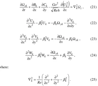
Substituting the cosine and sine transforms (Eq. 17 and 18) in the vorticity transport equations (11 to 13) and in the velocity Poisson equations (14 to 16) yields the governing equations in the Fourier space:
( )
x k k k k k k xk Ω h U β Re Go B β y A tΩ − 2 2 =∇2
∂ ∂ + ∂ ∂ , (19) Ωy x A C β t Ω k k k k
yk =∇2
( )
z k k k k zk Ω x U h Re Go -y C x B tΩ 2 2 =∇2
∂ ∂ ∂ ∂ + ∂ ∂ + ∂ ∂ , (21) y x V U x U k yk k k k k ∂ ∂ ∂ − Ω − = − ∂ ∂ 2 2 2 2 β
β , (22)
xk k zk k k k k x V y V x V Ω + ∂ Ω ∂ − = − ∂ ∂ + ∂ ∂ β β2 2 2 2 2 , (23) y V x W x W k k yk k k k ∂ ∂ + ∂ Ω ∂ = − ∂ ∂ β β2 2 2 , (24) where: − ∂ ∂ + ∂ ∂ = ∇ 2 2 2 2 2 2 1 k k y x
Re β . (25)
The Eqs. (19) to (24) were solved numerically in the domain shown schematically in Fig.3. An orthogonal, uniform grid, parallel to the wall was used. The fluid enters the computational domain at x=x0 and exits at the outflow boundary x=xmax. Disturbances were
introduced into the flow field using a suction and blowing function at the wall in a disturbance strip, located between x1 and x2.
Between x3 and x4 a buffer domain technique was implemented in
order to avoid wave reflections at the outflow boundary. A Blasius boundary layer was used as the base flow.
Figure 3. Integration domain.
Boundary Conditions:
At the upper boundary (y=ymax) the flow was assumed to be
irrotational. This is satisfied by setting all vorticity and their derivatives to zero. The velocity components are also set to zero.
0 and 0 = ∂ ∂ = y F ,
Fk , (26)
where Fk =
{
Uk ,Vk ,Wk ,Ωxk ,Ωyk ,Ωzk}
At the wall (y=0), no-slip conditions are imposed for the streamwise (Uk) and the spanwise (Wk) velocity components (Eq.
(27)). For the wall-normal velocity component (Vk) the
non-penetration condition is imposed for all points at the wall except between x1 and x2, where the disturbances are introduced as
explained below. In addition, the condition ∂ Vk /∂ y = 0 is imposed
to ensure conservation of mass.
0 for
0 =
=
=W y
Uk k , (27)
2 1 or and 0 for
0 y x x x x
Vk = = . (28)
The following equations are used for evaluating the vorticity components at the wall:
k k k yk xk k xk V y x x 2 2 2 2 ∇ − ∂ ∂ Ω ∂ − = Ω − ∂ Ω ∂ β
β (29)
k k k x k z V x 2 ∇ − Ω = ∂ Ω ∂
β . (30)
The introduction of the disturbances at the wall is done via a slot in the region (i1≤i≤i2), where i1 and i2 are the first and the last
point of the disturbance strip. The suction and blowing normal velocity variation along the streamwise direction is given by the function:
(
i ,0 ,t)
A sin3( )
for i1 i i2Vk = ∈ ≤ ≤
and
(
x ,0 ,t)
0 for i i1 and ii2Vk = (31)
where ε=π(i - i1) (i2 – i1 ) and A is a real constant that can be chosen
to adjust the amplitude of the disturbance. The chosen function (sin3) ensures that, at i = i
1 and i = i2, the normal velocity
component, its first and second derivatives do not have a discontinuity going in and out of the disturbance strip region. The variable i indicates the grid point location xi in the streamwise
direction, and points i1 and i2 correspond to x1 and x2 respectively.
At the inflow boundary (x = x0), the velocity and vorticity
components are specified based on the Blasius boundary layer solution.
( )
y =UBlasius, v( )
y =VBlasius, w( )
y =0u . (32)
( ) ( )
Blasius 00 y z z
x , w , w y w
w = = = . (33)
At the outflow boundary (x = xmax), the second derivative of the
velocity and vorticity components are set to zero:
0 2 2 = ∂ ∂ x Fk . (34)
A damping zone near the outflow boundary is defined in which all the disturbances are gradually damped down to zero. This technique is well documented in Kloker et al. (1993), where the advantages and requirements are discussed. Meitz and Fasel (2000) adopted a fifth order polynomium as damping function, and the same function is used in the present simulations. The basic idea is to multiply the vorticity components by a ramp function f2 (x) after
each integration step. This technique is very efficient in avoiding reflections that could come from the outflow boundary conditions when simulating disturbed flows. Using this technique, the vorticity components result:
(
x,y)
f( ) (
x k x,y,t)
k = Ω
Ω 2 , (35)
where Ωk (x,y,z) is the disturbance vorticity component that comes
out from the Runge-Kutta integration and f2 (x) is a ramp function
The implemented function was:
( )
( )
5 4 32x=f∈=1−6∈+15∈−10∈
f , (36)
where ε = (i – i3) / (i4 – i3) for i3≤i≤i4. The points i3 and i4
correspond to the positions x3 and x4 in the streamwise direction
respectively. To ensure good numerical results a minimum distance between x3 and x4 and between x4 and the end of the domain— x3
and xmax should be warranted. In the present simulations these zones
have 30 grid points each.
Another buffer domain located near the inflow boundary is also implemented in the code. As pointed out by Meitz (1996), in simulations involving streamwise vortices reflections due to the vortices at the inflow can contaminate the computation. The function adopted here is similar to the one used for the outflow boundary:
( ) ( )
5 4 33x=f∈=6∈−15∈ +10∈
f , (37)
where is ε = (i – 1) / (i1 – 1) for the range 1≤i ≤i1. All the
vorticity components are multiplied by this function in this region. Simulations with two different types of buffer domain close to the inlet boundary were carried out. In the first type, the function (37) was applied to all Fourier modes between x0 and x1. In the
second type, the damping function was used only for the fundamental Fourier mode in the region between x0 and x1. For the
other Fourier modes, all the vorticity components were set to zero between x0 and x2. In the second type of buffer domain, the damping
function was also used between x2 and 2x2 for all modes but the
fundamental. The reasons for using this technique is discussed in the presentation of results.
Numerical Method
The governing Eqs.(19) to (24) are solved using a compact high-order finite difference technique.
The solution is marched in time according to the following steps:
1. Impose initial conditions using a 2D solution for Uk, Vkand
Ωzk and set the other variables, Wk, Ωxk andΩyk, to zero;
2. Introduce disturbances at the wall through the disturbance strip;
3. Calculate the new vorticity distribution in the whole field, except at the wall, integrating Eq.(19) to (21);
4. Taper the vorticity disturbance components to zero at the damping zones near the inflow boundary and near the outflow boundary;
5. Calculate the wall normal velocity component (Vk) by
solving the V-Poisson equation - Eq.(23);
6. Calculate the streamwise velocity component (Uk) by using
Eq.(4) for the 2D mode and the U-Poisson equation - Eq.(22) for the others modes;
7. Calculate the spanwise velocity component (Wk) by using
the W-Poisson equation - Eq.(24);
8. Calculate the streamwise vorticity component at the wall by solving the Ωx-Poisson equation - Eq.(29);
9. Calculate the spanwise vorticity component at the wall by solving the Ωx-Poisson equation - Eq.(30);
10. Return to the second step until the desired integration time is reached.
The time derivatives in the vorticity transport equations were discretized with a classical 4th order Runge-Kutta integration scheme (Ferziger and Peric, 1997). The steps 4 to 9 are carried out for each Runge-Kutta time step.
The spatial derivatives were calculated using a centered, 6th
order compact finite difference scheme. For the boundary points one sided 5thorder approximation were used, while near the boundaries,
an asymmetric 6th order approximation was used (Souza et al.
2002a, Souza et al. 2002b). The discretization stencils are: For the points at the boundary (i=1):
(
)
( )
5 5 4 3 2 1 2 1 2 16 72 16 74 24 1 4 dx O f f f f f dx f f + + − + + ′ + ′ = ′ + ′ . (38)For the first grid line next to the boundary (i=2):
(
)
( )
6 5 4 3 2 1 3 2 1 30 80 760 300 406 120 1 2 6 dx O f f f f f dx f f f + + − + + ′ − ′ − = ′ + ′ + ′ . (39)For the interior points, a 6th order Padé approximation was used:
(
)
( )
6 2 1 1 1 1 28 28 12 1 2 3 dx O f f f f dx f f f i i i i i i i + + + + − − = ′ + ′ + ′ + + − + − . (40)The second derivative, at the boundary (i=1), was discretized using a 5th order asymmetric approximation:
(
)
( )
5 6 5 4 3 2 1 2 2 1 36 145 550 11170 20285 9775 120 1 137 dx O f f f f f f dx f f + + − − + + − = ′′ + ′′ . (41)The first grid line near the boundary (i=2), a 6th order asymmetric approximation was used:
(
)
( )
6 7 6 5 4 3 2 1 2 3 2 1 26 2176 810 2320 1890 8424 4834 360 1 3 12 dx O f f f f f f f dx f f f + − + − + + + − = ′′ + ′′ + ′′ . (42)The interior points were calculated with a 6th order Padé
approximation:
(
)
( )
6 2 1 1 2 2 1 1 3 48 102 48 3 4 1 2 11 2 dx O f f f f f dx f f f i i i i i i i i + + + − − + = ′′ + ′′ + ′′ + + − − + − . (43)At the opposite boundaries, i = N and i = N - 1, approximations similar to the ones used for the grid lines i = 1 and i = 2 were used.
The V-Poisson equation (23) was solved using a Full Approximation Scheme (FAS) multigrid (Trottenberg and Hackbusch, 1986). A v-cycle working with 4 grids was implemented. The number of cycles used varied according to the convergence criteria. The adopted criteria requires that the residue be less than 10-9. The residue of the V-Poisson equation is:
xk k zk k x V s
Re + Ω
∂ Ω ∂ − −∇
= 2 β . (44)
Code Verification and Validation
In order to test the accuracy and reliability of the mathematical model and numerical implementation, the experimental results of Swearingen and Blackwelder (1987) were compared to the numerical results. Results from the DNS model were also compared to the results obtained with other numerical models (Mendonça, 2000, Lee and Liu, 1992) for the same experiment (Swearingen and Blackwelder, 1987).
The experiment of Swearingen and Blackwelder (1987) considers a boundary layer on a concave plate with R=3.2 m with a free-stream velocity of U∞ = 5 m/s. The average spanwise
wavelength observed in the experiment is λz, =1.8 cm, which
corresponds to a non-dimensional wavenumber of β=34.90 and a wavelength parameter for the fundamental Fourier mode
Λf = (U∞λz / ν) (λz /R)1/2 = 450.
The reference length used was L=10 cm. The simulation started at x0 = 10 cm from the leading edge, which corresponds to a Görtler
number Go = 2.39, and a Reynolds number Re = 33124.
The number of grid points in the streamwise and wall-normal directions were 321 and 281 and respectively. The computational domain was 11.8 long and 0.231 tall. The disturbance-strip was located at 1.6 ≤ x ≤ 2.6. Seven Fourier modes were used in the simulation. Test runs with a smaller grid spacing and larger number of Fourier modes indicated that the solutions were grid independent.
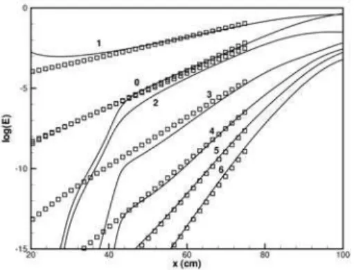
Figure 4 presents the streamwise development of the disturbance energy for each k Fourier mode. The disturbance energy is defined as:
0 k i dy w v u
Ek =∫0∞ k′2+ ′k2+ k′2 f > , (45)
and
0 k dy w u
Ek= ∫∞ k′ + k′ for >
2 1 0
2 2
, (46)
where u’, v’ and w’ are disturbance velocity components.
The disturbance energy of the mean flow distortion did not take into account the disturbance velocity component normal to the wall— v’0 to allow comparisons with the PSE model, where v’0 does
not go to zero as y→ ∞.
The comparison shows very good agreement between the DNS results and the PSE results for all Fourier modes. The difference observed in the region between the suction and blowing strip and x = 40 cm, corresponds to a receptivity region, where the wall disturbance slowly evolves to Görtler vortices.
Figure 4. Streamwise development of the disturbance energy of each Fourier mode. Comparison between PSE (squares) and DNS results (solid lines). Fourier modes 0 to 6.
Figures 5 and 6 show contours of the streamwise velocity component in the ( y, z ) plane. The numerical study from Lee and Liu (1992) and the measurements from Swearingen and Blackwelder (1987) are presented for the same streamwise positions. For the two different streamwise positions given, the results show a very good agreement for the development of the mushroom type structures. The experimental results at x = 110 cm indicate that the mushroom structures are already dissipating due to secondary instability effects. In the numerical simulation this effect was not present. Secondary instability only develops if a high frequency signal is also introduced in the flow field. In the absence of secondary instability the amplification of the vortices saturates as shown in Figure 4 after x = 90 cm. The numerical results from Lee and Liu (1992) are based on a 2nd -order model, being slightly more dissipative than the current one.
Figure 6. Same as Fig 5 for streamwise position x = 110 cm.
Results
In this section the boundary layer response to disturbances introduced in the flow field through a suction and blowing strip is investigated using direct numerical simulation. The study considers the relationship between the imposed wavelength in the suction and blowing strip and the resulting vortex wavelength. The initial development of the disturbances are studied in the receptivity region just after the disturbance strip. Only the primary instability mechanism is considered, therefore, high frequency disturbance signals to generate secondary instability were not introduced.
The boundary layer response to four different disturbance wavelength imposed in the suction and blowing strip was investigated. They correspond to wavelength parameters Λ of 56.25, 159.1, 450.0 and 692.6. The fastest growing mode has Λ=210 according to the LST.
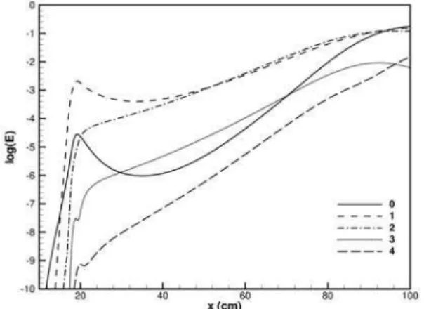
Figure 7 shows the mean flow distortion and other four Fourier modes kinetic energy variation along the streamwise direction of a disturbance introduced through the suction and blowing strip. The imposed wavelength corresponds to Λ=56.25. After an initial
receptivity region located between x = 18 cm and x = 24 cm, the disturbance propagates as centrifugal instability Görtler vortices. Although only a single Fourier mode was imposed in the suction and blowing strip, higher harmonic Fourier modes are excited in the receptivity region. The growth rate of the fundamental mode is small and the higher harmonic modes are stable according to linear stability theory. After the receptivity region, the growth of all Fourier harmonics are due to the growth of the fundamental mode in a non-linear process.
Figure 7. Streamwise development of the disturbance energy for ΛΛΛΛf=56.25. Fourier modes 0 to 4.
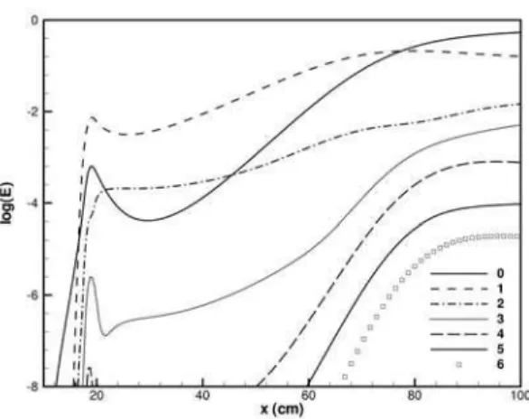
Similar results are obtained by changing the spanwise wavelength imposed at the disturbance strip to Λ = 159.1. The energy variation in the streamwise direction for different Fourier modes is shown in Fig. 8. Again, after an initial receptivity region the disturbance evolves to Görtler vortices further downstream. The typical GV mushroom structure at the streamwise position x = 100 cm is shown in Fig. 9.
Figure 8. Streamwise development of the disturbance energy for ΛΛΛΛf=159.1. Fourier modes 0 to 7.
Figure 9. Contour lines of streamwise velocity u/U∞∞∞∞ from 0.1 to 0.9 in increments of 0.1. Streamwise position x = 100 cm.
According to linear stability theory, GV with wavelength parameter greater then Λ = 56.25 have a weak amplification. The predominant forcing for this mode is the nonlinear GV with wavelength parameter Λ=159.1. That is the reason why GV with different wavelengths are not observed in the flow field, despite the strong initial amplification of the higher harmonics.
The third numerical simulation presented considers an imposed disturbance at the suction and blowing strip with a wavelength parameter Λf = 450. The flow parameters are those from the
Swearingen and Blackwelder (1987) experiment and the excited wavelength correspond to the experimentally observed wavelength.
The energy variation in the streamwise direction for different Fourier modes is presented in Fig. 12. The development of these modes are compared to the corresponding modes of a numerical experiment where the higher harmonics are suppressed in the receptivity region, as shown in Fig. 13. The main difference is in the development of the first harmonic, Λ=159.1. If this mode is not suppressed, it grows strongly beyond the receptivity region. According to LST this mode is unstable and both the fundamental mode and this mode are amplified by the centrifugal instability mechanism.
Figure 10. Streamwise development of the disturbance energy for ΛΛΛΛf=159.1 with higher harmonics suppression in the receptivity region. Fourier modes 0 to 7.
Figure 11. Contour lines of streamwise velocity u/U∞∞∞∞ from 0.1 to 0.9 in increments of 0.1 with higher harmonics suppression in the receptivity region. Streamwise position x = 100 cm.
Figure 12. Streamwise development of the disturbance energy for ΛΛΛΛf=450. Fourier modes 0 to 7.
Figure 13. Streamwise development of the disturbance energy for ΛΛΛΛf=450 with higher harmonic suppression in the receptivity region. Fourier modes 0 to 7.
Figure 16 corresponds to a numerical simulation for a suction and blowing disturbance with Λ = 692.6. The receptivity region goes from x = 18 cm to x = 40 cm. Again, the suction and blowing strip generates a range of Fourier modes. According to LST, the mode with Λ = 244.9 has a growth rate higher than that of the excited mode Λ= 692.6. After x = 50 cm, these modes have about the same energy level.
Since both modes are unstable according to LST, the centrifugal instability amplify both modes simultaneously. Consequently, the mushroom structure is strongly distorted when compared to the classic GV mushroom structure generated from a single mode. The resulting distorted mushroom structure can be observed in Fig. 17. The simultaneous growth of a mode with a spanwise wavelength that is half the imposed wavelength reinforces the up-wash region and creates two smaller up-wash regions on both sides of the original mushroom. This structure will probably have a completely different secondary stability characteristics.
Figure 14. Contour lines of streamwise velocity u/U∞∞∞∞ from 0.1 to 0.9 in increments of 0.1. ΛΛΛΛf=450 with higher harmonic suppression in the receptivity region. Streamwise position x = 110 cm.
Figure 15. Contour lines of streamwise velocity u/U∞∞∞∞from 0.1 to 0.9 in increments of 0.1. ΛΛΛΛf=450. Streamwise position x=110 cm.
Numerically suppressing the growth of other harmonics in the receptivity region allows a single mode to grow as shown in Fig. 18. This mode will cascade energy to higher harmonics further downstream an produce the classic GV mushroom structure as seen in Fig. 19.
Figure 16. Streamwise development of the disturbance energy for Λ
Λ Λ
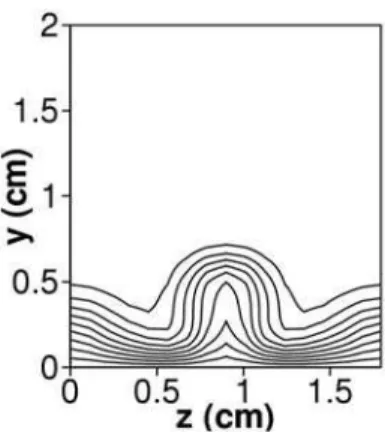
Figure 17. Contour lines of streamwise velocity u/U∞∞∞∞ from 0.1 to 0.9 in increments of 0.1. ΛΛΛΛf=692.6. Streamwise position x = 100 cm.
Figure 18. Streamwise development of the disturbance energy for Λ
Λ Λ
Λf=692.6. Higher harmonics suppressed. Fourier modes 0 to 4.
Figure 19. Contour lines of streamwise velocity u/U∞∞∞∞from 0.1 to 0.9 in increments of 0.1. ΛΛΛΛf=692.6. Streamwise position x = 100 cm.
A last simulation was done with three different disturbance wavelength imposed in the suction and blowing strip, Λ=450, Λ=159 and Λ=56.25, all with identical initial amplitudes. The spanwise variation of the normal velocity component at the wall is given by cos(βκz)+cos(2βκz)+cos(3βκz). The resulting streamwise
development of the disturbance energy is plotted in Fig.20. It can be observed that both the fundamental mode (mode 1) Λf = 450 and the
first harmonic (mode 2) Λ = 159.1, have a strong growth, and when mode 2 saturates, mode 1 continues to grow. It can also be observed that the Fourier mode 2 grows stronger than mode 1 in the region
between the streamwise positions x = 40 cm and x = 70 cm. In Figs. 21 and 22 the mushroom structure is plotted at two streamwise positions, x = 70 cm and x = 110 cm. At the streamwise position x=70 cm, where mode 2 dominates, three mushroom structures are observed. At the streamwise position of x = 110 cm, the modulated pattern is strongly pronounced. The structure is very different from the typical GV. In this case also, the GV will probably have a different secondary instability response.
Conclusions
The paper presents a numerical model based on a high-order compact finite difference scheme to solve the complete Navier-Stokes equations. This model is used in a direct numerical simulation of flows over concave surfaces. The model was verified by comparing results with three different numerical models (Mendonça, 2000, Li and Malik, 1995, Lee and Liu, 1992). The validation was done by comparing the results with experimental results from Swearingen and Blackwelder (1987).
Görtler vortices generated by disturbances introduced at the wall by suction and blowing in a disturbance strip may have a different structure from the one observed according to weakly nonlinear theory. This behavior is observed because the suction and blowing region excites different Fourier modes which may be unstable according to LST. This modes may have a growth rate higher than the growth rate of the fundamental imposed mode. The simultaneous growth of the different modes modifies the resulting mushroom pattern. This may have significant consequences to secondary instability, which is strongly dependent on the velocity profiles formed by the vortices.
In order to use the DNS model to study the weakly nonlinear development of Görtler vortices of a specified wavenumber, it was necessary in some cases to eliminate the undesired Fourier modes generated by suction and blowing. Future studies will be conducted in order to evaluate the secondary instability of the modified mushroom structures.
Figure 21. Contour lines of streamwise velocity u/U∞∞∞∞ from 0.1 to 0.9 in increments of 0.1. Streamwise position x=70 cm.
Figure 22. Contour lines of streamwise velocity u/U∞∞∞∞ from 0.1 to 0.9 in increments of 0.1. Streamwise position x = 110 cm.
Acknowledgments
The first author acknowledges the support received from the transition research group of the Institut für Aerodynamik and Gasdynamik (IAG) from Universitat Stuttgart, where he spent 6 months as a visiting scientist. The financial support received from FAPESP is also acknowledged.
References
Bippes, H. 1978. Experimental Study of the Laminar-Turbulent Transition on a Concave Wall in a Parallel Flow. Tech. rept. NASA TM— 75243. National Aeronautics and Space Administration – NASA.
Bottaro, A., and Luchini, P. 1999. Görtler vortices: are they amenable to
local eigenvalue analysis? Eur. J. Mech. B / Fluids, 18, 47–65.
Bottaro, A., and Zebib, A. 1997. Görtler Vortices Promoted by Wall
Roughness. Fluid Dynamics Research, 19, 343–362.
Ferziger, J. H., and Peric, M. 1997. Computational Methods for Fluid Dynamics. Springer. Springer–Verlag.
Floryan, J. M. 1991. On the Görtler Instability of Boundary Layers.
Prog. Aerospace Sci., 28, 235–271.
Görtler, H. 1940. ON the three-dimensional instability of laminar boundary layers on concave walls. Tech. rept. NACA TM-1375. National Advisory Commitee for Aeronautics – NACA.
Guo, Y., and Finlay, W. H. 1994. Wavenumber Selection and
Irregularity of Spatially Developing Nonlinear Dean and Görtler Vortices. J. of Fluid Mechanics, 264, 1–40.
Hall, P. 1982. Taylor-Görtler Vortices in Fully Developed or Boundary Layer Flows: linear theory. J. Fluid Mechanics, 124, 475–494.
Hall, P. 1990. Görtler Vortices in Growing Boundary Layer: the Leading Edge Receptivity Problem, Linear Growth and The Nonlinear Breakdown Stage. Mathematika, 37(74), 151–189.
Kloker, M., Konzelmann, U., and Fasel, H. 1993. Outflow Boundary
Conditions for Spatial Navier-Stokes Simulation of Transition Boundary Layer. AIAA Journal, 31(4), 620–628.
Lee, K., and Liu, J.C.P. 1992. On the Growth of the Mushroomlike Structures in nonlinear Spatially Developing Goertler Vortex Flow. Physics of Fluids, A4, 95–103.
Li, F., and Malik, M. R. 1995. Fundamental and Subharmonic Secondary Instability of Görtler Vortices. J. Fluid Mechanics, 297, 77–100.
Luchini, P., and Bottaro, A. 1998. Görtler vortices: a backward-in-time approach to the receptivity problem. J. Fluid Mechanics, 363, 1–23.
Meitz, H. L. 1996. Numerical Investigation of Suction in a Transitional Flat-Plate Boundary Layer. Ph.D. thesis, The University of Arizona.
Meitz, H. L., and Fasel, H. F. 2000. A compact-difference scheme for the Navier-Stokes equations in vorticity-velocity formulation. J. Comp. Phys., 157, 371–403.
Mendonça, M. T. 2000. Parabolized Stability Equations: A Review. In:
National Congress of Mechanical Engineering - CONEM 2000.
Myose, R. Y., and Blackwelder, R. F. 1995. Control of streamwise vortices using selective suction. AIAA J., 33(6), 1076–1080.
Myose, R.Y., and Blackwelder, R.F. 1991. Controlling the Spacing of Streamwise Vortices on Concave Walls. AIAA Journal, 29(11), 1901–1905.
Saric, W. S. 1994. Görtler Vortices. Ann. Rev. of Fluid Mechanics, 26, 379–409.
Souza, L. F., Mendonça, M. T. and Medeiros, M. A. F. 2001. A high resolution Navier Stokes solver for hydrodynamic stability analysis. In: 22nd CILAMCE, Iberian Latin-American Congress on Computational Methods in Engineering.
Souza, L. F., Mendonça, M. T. and Medeiros, M. A. F. 2002a. Assessment of Different Numerical Schemes and Grid Refinement for Hydrodynamic Stability Simulations. In: ENCIT 2002, 9th Brazilian Congress of Thermal Engineering and Sciences.
Souza, L. F., Mendonça, M. T., Medeiros, M. A. F., and Kloker, M. 2002b. Three Dimensional Code Validation for Transition Phenomena. In: ETT 2002, Third Spring School of Transition and Turbulence.
Swearingen, J. D., and Blackwelder, R. F. 1987. The Growth and Breakdown of Streamwise Vortices in the Presence of a Wall. J. Fluid Mechanics, 182, 255–290.