L. A. M. Riascos
L. A. Moscato
and P.E. Miyagi
Escola Politécnica da Universidade de São Paulo Depto. de Engenharia Mecatrônica e de Sistemas Mecânicos Av. Prof. Mello Moraes, 2231 05508-030 São Paulo, SP. Brazil [email protected]
Detection and Treatment of Faults
in Manufacturing Systems Based on
Petri Nets
This paper introduces a methodology for modeling and analyzing fault-tolerant manufacturing systems that not only optimizes normal productive processes, but also performs detection and treatment of faults. This approach is based on the hierarchical and modular integration of Petri Nets. The modularity provides the integration of three types of processes: those representing the productive process, fault detection, and fault treatment. The hierarchical aspect of the approach permits us to consider processes on different levels of detail (i.e. factory, manufacturing cell, or machine). Case studies considering detection and treatment of faults are presented, and a simulation tool is applied for verifying the models.
Keywords: Detection and treatment of faults, manufacturing systems, fault-tolerance, Petri nets
Introduction
Despite advances in automation technology, faults are events that cannot be ignored in a real manufacturing system. However, most reports in technical publications consider only the description and optimization of processes under normal conditions (Zhou and DiCesare, 1993). Thus, the development of a methodology that considers not only normal processes but also the detection and treatment of faults is essential for improving the flexibility and autonomy in manufacturing systems. 1
According to technical norms such as NBR 5462 of the Brazilian Association of Technical Norms (ABNT, 1994), a fault (Jalote, 1994) is in general defined as an interruption in the ability of an item to perform a specific function. In this paper, we adopt a more generic definition; i.e. the term fault is synonymous of failures, errors, mistakes, or disturbances that lead to undesirable or intolerable behavior of equipment.
Manufacturing systems are composed of different elements (such as machines, feeders, controllers, etc.); the interaction among these elements can be characterized as discrete, asynchronous, and sequential. Therefore, the process synchronization, deadlock avoidance, choice solution, etc. should be considered as the main issues in both normal and abnormal cases (Ho, 1992). An approach using Discrete Event Dynamic Systems (DEDS) allows us to consider these characteristics on the analysis and control of those systems. From this point of view, Petri Nets (PN) are employed as uniform techniques for modeling DEDS (Zurawski and Zhou, 1994).
This paper initially presents an overview of the main concepts related to detection and treatment of faults in manufacturing systems. In Section 3, a methodology that considers the detection and treatment of faults in manufacturing systems based on PN is introduced. In Section 4, case studies are presented in which the detection and treatment of faults in different hierarchical levels are modeled and analyzed. Finally, in Section 5, a simulator for PN, used to verify the models, is presented.
Nomenclature
AGV = Automated Guided Vehicle ANN = Artificial Neural Network BPN = Behavior Petri Net
Paper accepted January, 2004. Technical Editor: Edgar Nobuo Mamiya.
CAD = Computer Aided Design CAM = Computer Aided Manufacturing CNC = Computer Numerical Control CPN = Colored Petri Nets
DEDS = Discrete Event Dynamic System DPN = Distributed Petri Net
FMS = Flexible Manufacturing System PN = Petri Net
P/T PN = Place/Transition Petri Net
Petri Net Simbols I = vector of input arcs
M0 = vector of initial marking
O = vector of output arcs
P = vector of places Si = subnet i
T = vector of transitions
Tn = vector of normal transitions
TOR= vector of “OR” type transitions
Faults in Manufacturing Systems
The improvement of productivity in the field of manufacturing requires the automation of tasks and integration of techniques such as CAD and CAM. However, events such as start-up, maintenance, and faults cannot be treated completely automatically. In general, supervision by human operators is necessary, because the knowledge, experience, and skills for working with unexpected situations are very difficult to structure or reproduce. In addition, several reports confirm that totally automated machines are very expensive, and that appropriate combination of automated machines and human supervision is more effective for the operation of manufacturing systems when considering features such as fault-tolerance (Riascos and Miyagi, 2001; Miyagi and Riascos, 2002). Thus, in the automated manufacturing systems context, the balanced automation approach considering an appropriate level of automation is more effective than either totally automated machines or anthropocentric systems (Camarinha-Matos, 1996).
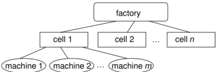
Manufacturing systems can be considered as distributed systems formed by several sub-systems, and can be organized according to a hierarchical structure (Figure 1):
The factory level: composed by production lines or manufacturing cells.
The manufacturing cell level: composed by machines. The equipment level: composed by specific devices forming
281
factory
cell 1 cell 2 cell n
machine 1 machine 2 machine m
…
…
Figure 1. Hierarchical structure of a distributed manufacturing system.
Both top-down and bottom-up approaches can associate the treatment of specific types of faults on different levels in a manufacturing system (Zhou and DiCesare, 1993).
Detection and Treatment of Faults
We are interested in the early detection of incipient faults, because it provides the means to schedule repairs before an actual fault takes place, (in contrast to corrective maintenance). The proposed methodology considers fault detection only on the equipment level while their treatment is executed on the most appropriated level.
Based on the automation degree of a manufacturing system, two types of fault detection on the equipment level can be considered (Frank, 1992):
Faults detected by monitoring a specific device parameter. For example, a leak of lubricant oil can be detected by installing a sensor, which monitors this parameter. In this case, a diagnosis is not necessary.
Faults that cannot be detected directly on the monitoring stage. For example, faults that need some type of diagnosis. This work focuses on faults of the second type.
In general, fault detection methods can be grouped into three categories (Frank, 1992):
Model-based: the actual and the expected behavior (from a mathematical model) are compared to identify a fault. Knowledge-based: qualitative models are associated with
heuristic symptoms for reasoning about fault causes.
Signal-based: such as spectral analysis that does not incorporate any model.
From a theoretical point of view, the model-based approach has reached a higher degree of maturity, particularly for controlling linear systems with small uncertainties. The challenge for designing a robust, model-based fault detection system is to generate measures insensitive to sources of uncertainties, but sensitive to actual faults. In the case of modeling with large uncertainties, a more suitable strategy is the knowledge-based approach. In fact, knowledge-based approaches have been applied successfully in fault detection (Frank, 1992).
In a knowledge-based approach, the detection and treatment of faults should consider several steps (Umeda et al., 1999).
1. Detection
1.1Data acquisition of operational parameters by sensors. 1.2Identification of the operational state (i.e. normal or
abnormal).
1.3Diagnosis of fault causes. 2. Treatment
2.1Proposition of a repair plan.
2.2Fault recovery or execution of a repair plan.
Fault Detection
The data extraction stage involves the machine's instrumentation, to measure a physical phenomenon (if possible,
without interfering with it). In general, the data acquisition is a continuous process and by itself cannot recognize an abnormal situation.
The identification stage concerns the analysis of the extracted data, to recognize binary states of a parameter (i.e. normal or abnormal). It includes discrepancy generation (between actual and expected data), and the evaluation of this discrepancy. The elimination of false alarms should also be performed at this stage.
The diagnosis stage is the reasoning process by which the causes of a fault are established. Diagnostic methods can be grouped into:
Symptom-based -- where knowledge about process history or statistical knowledge is organized in a framework of expert systems which associate the inputs with heuristic symptoms. Qualitative reasoning -- physical systems can be described by
a structure in order to determine its behavior from given initial conditions. The behavioral description can be a graph consisting of the possible states of the system (examples of this type of graphs are fault trees, causal networks, and Petri Nets for diagnosis).
The construction of a graph to describe those behaviors can be executed on two ways:
Based on human knowledge about the process, which establishes the relationship among variables and defines the criteria for choosing the next state.
Based on databases of records, where a probabilistic approach can be applied for searching the most probable belief-network structure (Cooper and Herskovits, 1992).
Fault Treatment
The fault treatment should be appropriate for each level of the manufacturing system (Hasegawa, 1996). On the equipment level, faults should be detected and, if possible, the broken machine should be recovered automatically.
The proposition of a repair plan concerns the selection of one procedure for recovering the machine from a fault. In general, several procedures can solve a specific problem. Thus, the best procedure should be selected based on two criteria: avoiding parameters off safe limits (i.e. applying mechanical and physical constraints), and avoiding side effects.
The fault recovery process can be executed in two ways: Adjusting operational parameters without changing or
reorganizing the logical structure of the machine. This approach is effective when actuators can be controlled to recover (totally or partially) the requested functions
Utilization of redundant resources. However, this type of redundancy can result in undesirably low-performance, high-cost, weight, and complexity.
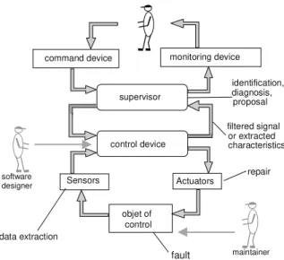
Figure 2 depicts the structure of a fault-tolerant machine based on the adjustment of operational parameters. Note that faults are assumed to occur only on the object of control. In general, human interaction is considered on the command and monitoring devices to make decisions during normal processes, start-up, or fault recovery processes. Human interaction can also be performed on the programming (on the controller) and maintenance (on the object of control).
control device
Actuators Sensors
objet of control
filtered signal command device monitoring device
or extracted characteristics supervisor
data extraction
identification,
repair
fault
diagnosis, proposal
software designer
maintainer
Figure 2. Structure of a fault-tolerant machine.
When a problem occurs on the manufacturing cell level, the first step in the fault treatment is to identify other equipment in the same cell which executes entirely, or partially the functions of the inoperative equipment. Then, the cell's load/unload device should modify the flow of parts until the inoperative equipment returns to the normal state (Hasegawa, 1996).
On the factory level, the fault treatment is executed by rescheduling the routes of material flow among cells. In Barros et al. (1997), an approach based on Place/Transition Petri Nets (P/T PN) and Colored Petri Nets (CPN) is presented considering fault-tolerant procedures for developing a supervisor in a Flexible Manufacturing System (FMS) based on the rescheduling of vehicle routes.
A methodology, which provides the means to model a system considering detection and treatment of faults, and to analyze the properties of different solutions, is essential for the design and implementation of more flexible and autonomous manufacturing systems. In this context, PN is viewed as a powerful tool for modeling and analyzing a manufacturing system on a DEDS point of view.
Integration of Modules for Fault Treatment in Manufacturing Systems
Petri Nets (PN) have been extensively used to model and analyze manufacturing systems (Zurawski and Zhou, 1994). One of the major advantages of using PN models is that the same model can be used for the analysis of behavioral properties and performance evolution, as well as for the systematic construction of discrete event simulators and controllers.
Based on Hasegawa (1996), PN have the following advantages: The ability to naturally represent the synchronization of
processes, the concurrence of activities, the presence of conflicts, causality, resource sharing, mutual exclusion, etc inherent characteristics of manufacturing systems.
Locality of states and actions, providing system monitoring in real-time requirements.
Interpretability (the possibility of associating objects of different meaning according to the purpose of the model e.g. validation, performance, and scheduling).
Adequate representation of a system's essential features, selecting an appropriate detail level. PN permit the construction of models applying top-down and bottom-up approaches.
As a graphical tool, PN permit effective visual communication, improving the communication between designers and costumers, thus avoiding complex specifications, ambiguous textual description, or specific mathematical notation which are generally difficult to understand.
As a mathematical tool, PN can be described by algebraic equations opening the possibility for formal analysis of the model. Thus, formal properties can be analyzed to identify specific characteristics like overflows and deadlocks. These advantages justify the use of PN in a methodology for modeling and analyzing manufacturing systems considering detection and treatment of faults.
A methodology is a collection of methods, and a method is a process for the construction of models. Therefore, the methodology proposed is a collection of methods for organizing the problem of modeling normal procedures, detection, and treatment of faults on both a vertical and a horizontal structure. On the vertical structure, a manufacturing system is organized in hierarchical levels (i.e. factory, cell, and equipment). On the horizontal structure, three modules are considered: normal processes, fault diagnostic, and fault treatment. A specific and adequate type of PN represents each module. In this context, the Distributed Petri Net (DPN) is introduced as a framework to integrate different types of Petri Nets, and to consider the three modules applying the same formalism (Riascos, 2002). The modules are as follows:
Module of normal processes represents the normal evolution of the productive process in a manufacturing system. In this research, this model is called central-PN, which is based on P/T PN.
Module of fault diagnosis the diagnostic execution of faults is based on the inverse interpretation of a cause-effect fault tree where the roots define the fault treatment and the leaves are the sensor states. This research applied the Behavior Petri Net (BPN) approach for modeling the diagnostic procedure (Portinale, 1997).
Module of fault treatment this module is based on the method introduced by Zhou and DiCesare (1993), in which subnets of P/T PN are added to the central-PN forming the Extended-central-PN (E-central-PN). Each subnet represents the treatment for each specific fault. The result on the fault diagnostic model (i.e. BPN) defines which sub-net is executed for an appropriate fault treatment.
Formally, a DPN can be defined as a quintuple DPN=(P,T,I,O,M0), where:
P = {p1,p2,... ,pm} is a finite set of places, where m∈IN is the
number of places,
T = Tn∪TOR = {t1,t2,... ,ts} is a finite set of transitions, where
s∈IN is the number of transitions and Tn ∩TOR = ∅,
I(pj,ti) = kji where kji∈IN is a constant that specifies the
relationship (i.e. the weight of the oriented arc) from pj to ti,
O(ti,pk)=kikspecifies the relationship (oriented arc) from ti to
pk,
M0 is the initial marking.
Tn is a “normal” transition defined in P/T PN (Murata, 1989), and TOR is a macro-transition defined in the context of BPN to
model the logical connective OR (Portinale, 1997). Figure 3 shows the equivalence between transitionsTOR and transitionsTn.
283
TOR
place
Tn Tn Tn
oriented arc inhibitor arc
Figure 3. Equivalence between transition TOR and normal transitions (adapted from Portinale, 1997).
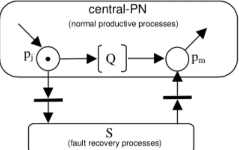
The modeling of fault treatment is based on the augmentation of fault treatment procedures in a PN model where initially those processes were not considered (Zhou and DiCesare, 1993). This approach provides the maintenance of several properties of the PN model, such as boundedness, safeness, liveness (absence of deadlock), and reversibility (re-starting). Figure 4 shows a subnet S added to central-PN based on the approach defined in Zhou and DiCesare (1993). The analysis of these properties is essential for verifying and improving the manufacturing system specifications.
The maintenance of such properties is guaranteed by the theorems introduced in Zhou and DiCesare (1993).
In a DPN, two types of transition firing rules should be considered, the transition firing on the E-central-PN and the transition firing on BPN blocks.
The firing rule of an enabled transitiont in the E-central-PN is the same rule of P/T PN. A firing of an enabled transition(ti∈Tn) removes from each input placepj (where I(pj,ti)>0) the number of
tokens equal to the weight of the oriented arcI(pj,ti) connecting pj to
ti. Basically a transitionti∈Tn is enabled to fire iff: M(pj) ≥I(pj,ti).
On the other hand, a model in BPN should be constructed from fault causes to effects (cause→effect). But, with diagnostic reasoning (instead of predictive reasoning), causes should be diagnosed based on the monitored effects (effect→cause). Thus, on BPN models, an inverse firing procedure should be considered (Portinale, 1997).
In a DPN structure, two types of formalisms should be considered: P/T PN and BPN. It implies in two separate analyses. Figure 5 depicts the integration of modules using DPN. Note that the connection between blocks for diagnostic execution (i.e. BPN) and E-central-PN is based only on procedures.
The P/T PN part is a mathematical tool with a graphic representation that facilities its use in the process monitoring by a human supervisor. The BPN part is a representation of fault diagnosis in machining processes which permits a clean and easy identification of abnormal situations; this understanding is essential to decision-making about the fault recovery process.
S pj
central-PN
Q pm
(normal productive processes)
(fault recovery processes)
Figure 4. Modeling of fault treatment based on the addition of subnets (adapted from Zhou and DiCesare, 1993).
central-PN Sub-net S1 Sub-net S2
Sub-net Sm
BPN1
BPN2
BPNn
E-central-PN
DPN
P/T PN BPN
Figure 5. Structure of integration based on DPN.
The construction of a model considering detection and treatment of faults can be structured in a sequence. The sequence, to apply the proposed methodology based on DPN, is as follows:
1. To identify “normal” activities of the process.
2. To model the sequence of “normal” activities in PN and to associate the resources to these activities, (it defines the central-PN).
3. To define faults and their treatment.
4. To model the fault treatment in subnets of PN and to define the E-central-PN.
5. To model the fault diagnostic process.
6. To associate the state (marking) in the E-central-PN and the state (marking) in the fault diagnostic model.
The next section presents case studies, to illustrate the application of the proposed methodology.
Case Studies
To illustrate the proposed methodology, case studies of detection and treatment of faults in manufacturing systems are considered. These case studies analyze a manufacturing system composed of one manufacturing cell. Two machines, one manipulator robot, and one Automated Guides Vehicle (AGV) compose the system (see Figure 6).
In Case 1, faults on the machining process are considered. In Case 2, faults on the load/unload processes are considered. In Case 3, faults on the AGV are considered. And, in Case 4, fault treatment considering the integration among equipment is considered.
Faults in the Machines
In the proposed methodology, the first step is to identify the “normal” activities: loading machine, machining, and unloading machine.
The second step is to model these processes through PN. The model of the processes is presented in Figure 7.
The third step is to identify the faults. Initially, faults in the machining process are considered.
M1 M2
robot
buffer input
buffer output
AGV
loading machine machining unloading machine
Figure 7. Manufacturing process modeled with PN (central-PN).
Case 1: Detection and Treatment of Faults in Machining Operations.
Different researchers prove that fault detection in machining processes can be structured in an automatic way (Cunha, 2000; Dornfeld, 1990; Santos, 1998). In this case study, faults by tool-wear, tool-break, and erroneous programming of machining parameters are considered. In general, the treatments for these faults are tool-change or parameter-change.
The fourth step is to model the fault treatment by subnets of PN and to define the central-PN. Figure 8 shows the resulting E-central-PN. The subnets represent the fault treatments by tool-change (S1), parameter changes (S2), and human intervention (S3).
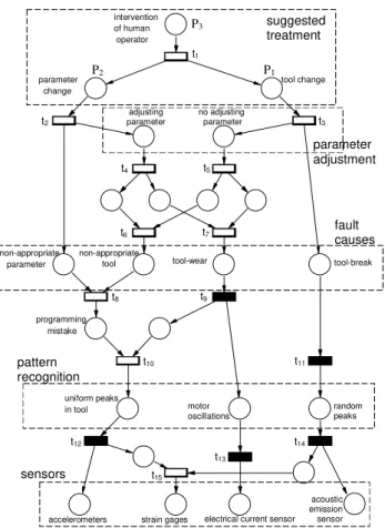
The fifth step is to define the BPN, to model the fault diagnostic process. The model of the diagnostic process is presented in Figure 9. Five layers compose the structure for fault diagnosis: sensors, pattern recognition, fault causes, parameter adjustment, and suggested treatment. The characteristics of each layer are the following:
Layer of Sensors: In this case, 1 sensor of electrical current, 3 accelerometers, 4 strain gages, and 1 sensor of acoustic emission constitute the data extraction system. The signals of these sensors are collected by an acquisition signal system, which recognizes tool states (normal or abnormal).
The accelerometers detect mechanical vibrations in the machine structure, which are produced by oscillations of cutting force (Santos, 1998).
The sensor of current detects variations in the current consumed by the electrical motor and relates it with the tool and workpiece condition (Santos, 1998).
The strain gages detect tool flexion or tool torsion (Cunha, 2000).
loading machine
unloading machine
change parameters discarding
broken tool
machining a new tool
does not exist
installing new tool
human operator verifying a fault
central-PN
S1
S2
S3
p1 p
2
p3
Figure 8. E-central-PN of a manufacturing system.
P3
P2 P1
sensors pattern recognition
fault causes suggested treatment
parameter adjustment
strain gages
acoustic emission sensor electrical current sensor uniform peaks
in tool random
peaks oscillations
motor mistake
programming parameter
non-appropriate non-appropriate
tool-wear
tool tool-break
parameter change
tool change intervention
of human operator
accelerometers
parameter adjusting
parameter no adjusting
t1
t2 t3
t4 t5
t6 t7
t8 t9
t10 t11
t12
t13
t14
t15
Figure 9. BPN model for fault detection in machining operations.
The acoustic emission sensor detects acoustic effects of stress waves for tool break detection (Byrne et al., 1995). Dornfeld (1990) and Santos (1998) prove the applicability of Artificial Neural Networks (ANN) for identifying tool conditions in a machining process. ANN were used to make data fusion of sensor signals with machining parameters such as speed, feed, and slop. Figure 10 shows the signal-processing structure representing the data acquisition and identification stages.
accelerometers PN-place
Sequential Forward Coding
filtering
axle x axle y axle z feed axle parameters
freq. (Hz)
LED
SG +
-strain gages PN-place
parameters
T
(N
m
)
t (seg.)
electrical current sensor PN-place
Linear Predictive Coeff. parameters
I
(a
m
p
.)
t (seg.)
A
acoustic emission sensor PN-place
+
-parameters
R
M
S
t (seg.)
285
Pattern Recognition: the signal peaks generated by the tool can be approximately uniform or totally random.
Signals with random peaks indicate tool-break or very high tool-wear. In these instances, the tool should be changed.
Signals with “uniform” peaks indicate slight tool-wear or CNC programming mistakes. In these instances, the process can be corrected through either tool change or parameter adjustments such as adjusting speed, feed, or slop.
Fault Causes: the causes of a fault are attributed to tool-wear, tool-break, or programming mistakes like applying a non-appropriate tool or erroneous machining CNC parameter. Faults from non-appropriated tools or erroneous parameters generate “uniform” peaks. Faults due to tool-wear are identified by motor oscillations and “uniform” peaks. Faults resulting from tool-break generate random peaks.
Parameter Adjustment: faults caused by slight tool-wear or non-appropriate tools can be corrected by adjusting the machining parameters. This procedure is specified as follows:
1. The discrepancy between the actual and expected behavior is calculated based on characteristic extraction from signal sensors.
2. Parameter adjustments are defined to correct this difference. In general, several parameter adjustment combinations can solve the problem; in this case, the best combination based on steps 3 and 4 should be selected.
3. Unsafe parameters are avoided. The safe parameters are based on mechanical and physical constrains of equipment, machining process, tool, workpiece, etc. The combinations with unsafe parameters should be eliminated.
4. Side effects are avoided. In this case, the system should select a parameter adjustment with the least side effects. If necessary, a second parameter adjustment should be generated to eliminate the side effects Suggested Treatment: this layer indicates the treatment to
recover the machine of a fault. The treatments are toolchange (placep1), parameter change (p2), or human intervention (p3).
There are cases where the automatic treatment by tool change or parameter change cannot be successful, so the sensors still indicate a type of abnormal situation. The system then considers intervention of a human operator if, after a second tool-change or k-th parameter-changes, the fault cannot be corrected. Those conditions are verified applying a delay. The net in Figure 9 is safe, non-cyclic, and non-conflict according to BPN characteristics (Portinale, 1997). In this model, the transition firing is based on two criteria: transitions Tn fire immediately after being enabled, and transitionsTORfire according to input or output conditions (t1,t2,t3,t4,t5 fire with at least one
output condition, and t6,t7,t8,t11,t15fire based on specific criteria).
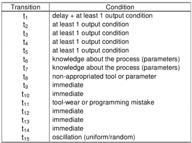
Table 1 describes the criteria for transitionfiring on the BPN of Figure 9.
The final step in the methodology is to associate the marking on places in the BPN part and the marking in the E-central-PN. This association permits us to connect the conclusion of the diagnosis
(p1, p2, and p3) and the choice of a fault treatment to recover the
system (tool change (p1), parameter changes (p2), or human
intervention (p3)). The marking on places in the suggested treatment
layer on the BPN (Figure 9) defines the flow of tokens in the central–PN and the execution of a subnet (Figure 8).
Table 1. Criteria for transition firing of the BPN (Figure 9).
Transition Condition t1 delay + at least 1 output condition
t2 at least 1 output condition
t3 at least 1 output condition
t4 at least 1 output condition
t5 at least 1 output condition
t6 knowledge about the process (parameters)
t7 knowledge about the process (parameters)
t8 non-appropriated tool or parameter
t9 immediate
t10 immediate
t11 tool-wear or programming mistake
t12 immediate
t13 immediate
t14 immediate
t15 oscillation (uniform/random)
Case 2: Faults in Load and Unload Processes
The load or unload operations can be analyzed like assembly or disassembly operations based on a sequence of discrete events (McCarragher, 1994).
Applying the proposed methodology, the first step is to identify “normal” activities. For a better explanation, the load or unload processes are separated onto three activities: grasping, transporting, and release.
Grasping is the initial approximation for catching the workpiece. In the load process, it is caught from the input buffer to the machine. In the unload process, it is caught from the machine to the output buffer.
Transporting is to firmly support and to move the workpiece close to the final position.
Release is to leave the workpiece. In the load process, the workpiece is left on the machine; and, in the unload process the workpiece is left on the output buffer.
The second step is to model the sequence of “normal” activities in PN and to define the central-PN. The central-PN is presented in Figure 11.
P0A
P2A
P1A
transporting
P1C
P2C
P0C
Px Py
Pz
P4
P4
P4
P4
P4
arriving part
grasping
begin transport
begin machining
release begin release
S1
S2
S3
central-PN
The third step is to identify the faults. In the transporting activity, faults such as crashing with an obstacle and the fall of the workpiece are considered. In the grasping and release activities, faults associated with inappropriate positioning/assembly procedure are considered.
The fourth step is to model the fault treatment by sub-nets of PN and to define the E-central-PN.
The fault treatments in the grasping and release activities are modeled applying the approach described in McCarragher (1994). In these activities, a token on the place p0 represents the initial
approximation to the workpiece before any type of contact. A token on the place p1 represents a state where the activity is executed
unsuccessfully or a “faulty” state. A token on the placep2 represents
a state where the activity is executed successfully, or a “normal” state.
In the transporting activity, a token on the placepx represents
the execution of a new trajectory avoiding an obstacle. A token on the placepy, represents the total fall of the workpiece. A token on
the place pz, represents the continuation of transporting activity.
Figure 11 shows the resulting E-central-PN.
The fifth step is to model the operational state (normal or faulty) of the equipment. Sensors in the robot’s grip or wrist (robot = load/unload equipment) can monitor the load (or unload) process. Crashing effects can be recognized from discrepancies between sensor signals and kinematics/dynamics effects (Asada and Slotine, 1986). Figure 12 shows a simplified representation of the operational state of the equipment.
The final step is to associate the marking on places in the model of equipment (Figure 12) and the marking in the E-central-PN (Figure 11). In this case, the association was performed by inhibitor-arcs (Zurawski and Zhou, 1994).
Case 3: Detection and Treatment of Faults in AGVs
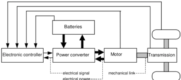
An AGV is a transporter using a navigation system for controlling its movements. Generally, electrical motors propel it. Faults in the navigation system of AGVs are analyzed in Král et al. (2000) and Preucil et al. (2000). A synthesis about the functional structure of AGVs as an electrical vehicle is introduced in Chan and Chau (1997). Figure 13 depicts the structure of the electric propulsion system where thick arrows represent power flows, and thin lines represent signal flows.
Applying the proposed methodology, the first step is to identify the “normal” activities. The activities are loaded, unloaded, stopped, and parking.
Loaded is an AGV transporting cargo: generally a pallet with workpieces.
Unloaded is an AGV in movement, but without cargo. Stopped is an AGV waiting (stopped) for a transportation
requirement.
Parking is an AGV in the parking area. In this area, the battery charging process can be executed.
P4 (normal process)
P5 (faulty process)
Figure 12. Simplified model of load/unload state.
Electronic controller Power converter Motor Transmission
Batteries
electrical signal electrical power
mechanical link
Figure 13. Functional diagram of an electric propulsion system (adapted from Chan and Chau, 1997).
The second step is to model these activities in PN defining the central-PN. The sequence of these activities is represented in Figure 14. In this model, the firing of transitions t1 and t2 represents the
respective load and unload processes of cargo on the AGV. The third step is to determine the faults and the fault treatment. The faults considered are battery discharge, short-circuits in the electrical motor, and mechanical friction. In this case, the recommended treatments to recover the equipment are immediate battery charging and corrective maintenance.
The fourth step is to model the fault treatment in subnets of PN and to define the E-central-PN. Figure 14 depicts the fault treatment. This model is composed of a central-PN and two sub-nets representing fault treatment by maintenance (S1) and battery
charging (S2).
Maintenance is an AGV in the maintenance area. In a fault case, an AGV is generally undercharged enough to maintain operation for a while, to finish its work, and to move by itself to the maintenance area.
Battery charging is an AGV in the parking area making a battery charge.
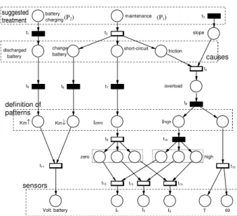
The fifth step is to construct the BPN for modeling the fault diagnostic process. Figure 15 shows the BPN for fault diagnosis in an AGV propelled by electrical motor. In this case, four layers compose the model: sensors, definition of patterns, fault causes, and suggested treatment.
For industrial applications, generally three-phase motors propel AGV and a type of fault can take place when only one current becomes zero. The following gives a short description of each layer:
loaded
unloaded
parking stopped
maintenance
t1 t2
t3 t4
t5
t6
t8
t9
t7
t11
t10
battery charging
P2
P1
S1
S2
central-PN
287
suggested treatment
causes
sensors definition of patterns
battery charging
t1
discharged battery
t5
Km↑
t11
Km↓
Volt. battery
zero high
t13
t12 t14
I1 I2 I3
t9 t10
short-circuit t2
maintenance
change
battery friction
Ihigh
t8
overload t4
t15
T ω
t6
slope t3
Izero
t7
(P1)
(P2)
Figure 15. Model in BPN for fault detection in an AGV.
Sensors− the placesbattery voltage, stator currents (I1, I2, and
I3), torque (T), and velocity (ω) compose the layer of sensors. A
token in one of these places indicates a variable off expected limits. Therefore, four types of sensors (voltmeter, ammeters, torque sensor, and encoder) compose the data extraction system. The signals of these sensors are collected by an acquisition signal system, which recognizes every normal or abnormal operational state (Altug et al., 1999).
Definition of Patterns − problems in battery charging are determined in this layer. A token on the place Km↑↑↑↑ means agreement between route length and one battery charging. A token on the place Km↓↓↓↓ means a poor route length for a battery charging. In this layer, problems in the three-stator currents are also identified such as short-circuit in one phase (transition t10) or overload in all currents (I1AND I2AND I3),
where the condition AND is represented by transitiont9.
Fault Causes− battery discharging, “permanent” problems in the battery (or alternator), short-circuits in at least one phase, and mechanical friction. Mechanical friction is generally associated with transmission, or with worn or broken bearings. Fault causes by mechanical friction can be confused with “normal” overloads (effects such as reduction of angular velocity or increasing of electrical current can be similar). For example, an AGV ascending a slope (a normal overload) is not associated with fault causes, and therefore the place slope
is off fault cause layer.
Suggested Treatment − in a case of battery discharge, immediately charging the battery is recommended (p2). In
other cases such as “permanent” battery problems OR short-circuit OR mechanical friction (the condition OR is represented by transition t2), the AGV should be removed
from operation and sent to maintenance area (p1).
The final step of the methodology is to associate the marking of places in the BPN (Figure 15) and the marking in the E-central-PN (Figure 14). This association establishes a linkage between the model of fault diagnosis and the E-central-PN.
Case 4: Faults in the Manufacturing Cell Level
On this level, the operational state and the interaction among equipment composing the manufacturing cell are considered.
Applying the proposed methodology, the first step is to identify “normal” activities. The machines can process 3 types of workpieces (w1, w2, and w3). The workpieces w1 are processed in
M1. The workpieces w2 are initially processed in M1 and then in
M2. The workpieces w3 are processed only in M2.
The second step is to model the activities in PN. Figure 16 represents the sequence of activities and the type of workpieces to be processed.
The third step is to determine the most important faults and their treatment. In this step, only faults in the machines are considered. In the event of a machine breaking, the processing of workpieces should be interrupted to execute the fault recovery; but, if possible, a predictive maintenance is considered when M1 or M2 have finished the process on the workpiece.
The fourth step is to model the fault treatment in sub-nets and to define the E-central-PN. Figure 16 depicts two subnets for fault treatment in M1 (S1 and S2) and two subnets for M2 (S3 and S4). S1
(S3) represents the fault treatment when M1 (M2) breaks; an
immediate recovery action should be executed. S2 (S4) represents a
fault treatment by predictive maintenance procedures, which permit it to finish the process by M1 (M2) on the workpiece.
The fifth step is to model the fault detection process. Figure 17 is a simplified representation of operational estates of M1 (left side) and M2 (right side). The marking evolution of these blocks can be based on the result of a fault diagnosis modeled in BPN.
The final step is to associate the marking on places in the operational state part (Figure 17) and the marking in the E-central-PN (Figure 16).
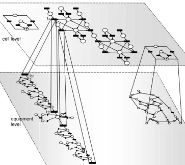
Top-down and bottom-up approaches can associate detection and treatment of faults considering hierarchical levels in a manufacturing system. For example, in Figure 18 the model on the manufacturing cell level (upper plane) and models on the equipment level (bottom plane) are associated. Note that activities can be unfolded on the lower level (for example, load/unload machine) or simplified on the upper level; therefore, specific types of faults can be considered according to the level analyzed.
P7
P8
P16
P17
P10
P9
P11
P12 P14
P13
P15
P18
P20
P21
P22
P19
t1
load-M1
unload-M1
load-M1 t2
load-M2
unload-M2 unload-M2
load-M2 t3
P1
P1
P4
P4 S1
S3
S2
S4
central-PN
P1 (M1-normal) P2 (M1-fault)
P3 (M1-maintenance) P6 (M2-maintenance)
P5 (M2-fault)
P4 (M2-normal)
Figure 17. Model of operational states of machines.
The dynamic behavior in models on different hierarchical levels is associated through the marking evolution. The marking evolution on one level affects the enable/disable condition on other levels. For example, in Figure 18 the firing of transitiont4 (cell level) begins
when transition t20 (equipment level) has fired, and the firing of
transitiont4 ends when transitiont25fires.
DPN Simulator
A simulation tool to edit and to analyze DPN was developed to verify the models (Takada, 1998). The program can simultaneously simulate several Petri Nets with linked procedures. The programming language uses graphic resources. Elements (such as places, transitions, and arcs) are edited by a “click” of mouse, and dialog boxes permit it to define properties and specifications of simulation. The software was developed for MS-Windows to use a friendly and well-known environment.
Case studies of fault-tolerant systems (such as cases 1, 2, 3, and 4) were verified showing compatibility between the dynamical behavior of every model and the expected behavior. The expected behavior is based on analytical methods individually applied to each graph. The structure of models was verified validating readability and accompanying the system evolution based on marking evolution on separated graphs.
cell level
equipment level
t4
t20
t25
Figure 18. Integration of models in the cell and equipment level applying top-down and bottom-up approaches.
Figure 19. Hard copy of simulator for case 1.
Figure 19 shows a hard copy of the simulator where the model for case 1 (faults in machining processes) was analyzed. The models for cases 2, 3, 4, and others were also analyzed in the simulation tool (Riascos, 2002).
The E-central-PN is based on P/T PN, and the BPN is based on the inverse firing procedure. To avoid the problem of two nets with different formalisms in the same simulator, the complement net (Miyagi, 1996) of the BPN is drawn in the simulator. Note that in the BPN part (upper net on Figure 19) the orientation of arcs has been inverted.
Conclusions
A methodology for modeling manufacturing systems based on Petri Nets (PN), and considering a hierarchical and modular approach for detection and treatment of faults was introduced.
The modules represent normal productive process, fault detection, and fault treatment. The central-PN based on Place/Transition Petri Net (P/T PN) represents the normal processes, Behavior Petri Net (BPN) represents the fault diagnosis, and subnets of P/T PN represent the fault treatment.
Case studies considering detection and treatment of faults, on the equipment and cell levels, illustrate the application of the methodology. They show the possibility of integration of distributed procedures on different nets, which can be associated on hierarchical levels (i.e. a manufacturing system composed by a set of machines distributed on several manufacturing cells).
One of the major problems of PN is to model large and complex systems due to the exponential explosion of the number of elements (such as places, transitions). The proposed methodology permits the analysis of models for detection and treatment of faults with a more rational and systematic method. In fact, formal properties of a PN model (such as reachability, liveness, safeness, choice free, etc.) can each be analyzed separately.
In Riascos (2002), an analytical analysis of the models in DPN was compared with traditional approaches in PN (Zurawski and Zhou, 1994) proving the advantages of the proposed methodology.
Acknowledgements
289
References
ABNT, 1994, “NBR 5462 Reliability and Manutenability”, (In Portuguese), ABNT, São Paulo, SP.
Altug, S.; Chow, M.; and Trussell, H.J., 1999, “Fuzzy Inference Systems Implemented on Neural Architectures for Motor Fault Detection and Diagnosis”, IEEE Transactions on Industrial Electronics, Vol.46, No.6, pp.1069-1078.
Asada, H.; and Slotine, J.E., 1986, “Robot Analysis and Control”, Wiley-Interscience Pub.
Barros, T.C.; Figueiredo, J.C.A.; and Perkusich, A., 1997, “A Fault Tolerant Colored Petri Net Model for FMS”, Journal of the Brazilian Computer Society, Vol.4, No.2.
Byrne, G.; Dornfeld, D.A.; Inasaki, I.; Ketteler, G.; König, W. and Teti, R., 1995, “Tool Condition Monitoring. The Status of Research and Industrial Application”, Annals of CIRP, Vol.44, No.2.
Camarinha-Matos, L.M., 1996, “Balanced Automation Systems”, Studies in Informatics and Control, Vol.5, No.2, pp.87-88.
Chan, C.C.; and Chau, K.T., 1997, “An Overview of Power Electronics in Electric Vehicles”, IEEE Transactions on Industrial Electronics, Vol.44, No.1, pp.3-13.
Cunha, V.L.C., 2000, “End Mill Sensor System for Tool Condition Monitoring”, (In Portuguese), M.Eng. Dissertation, Escola Politécnica da USP. São Paulo, SP, 136p.
Cooper, G.F.; and Herskovits, E., 1992, “A Bayesian Method for the Induction of Probabilistic Networks from Data”. Machine Learning,, No.9, pp. 309-347.
Dornfeld, D.A., 1990, “Neural Network Sensor Fusion for Tool Condition Monitoring”, Annals of the CIRP, Vol. 39, No.1, pp.101-105.
Durfee, E.H., 2001, “Distributed Problem Solving and Planning”, Multi-Agent Systems and Applications: ICAI 2001, 9th ECCAI, EASSS 2001,
Prague. In: Luck, M; Marik, V.; Stepánková, O.; and Trappl, R. (Eds.), Springer-Verlag, pp.118-149.
Frank, P.M., 1992, “Principles of Model-Based Fault Detection”, Proceedings of the International Symposium on AI in Real-time Control, Delft, pp. 363-370.
Hasegawa, K., 1996, “Modeling, Control and Deadlock Avoidance of Flexible Manufacturing Systems”, 11th Brazilian Congress of Automatics
(SBA), São Paulo, SP, pp.37-51.
Ho, Y-C. (Ed.), 1992, “Discrete Event Dynamic Systems: Analyzing Complexity and Performance in the Modern World”, IEEE Press, New York. Jalote, P., 1994, “Fault Tolerance in Distributed Systems”, Prentice-Hall.
Král, L.; Kulich, M.; Preucil, L.; and Stepán, P., 2000, “Complex System for Mobile Robot Navigation (COSYNA)”, The Gerstner Laboratory, Czech Tech. Univ., Prague.
McCarragher, B., 1994, “Petri Net Modelling for Robotic Assembly and Trajectory Planning”, IEEE Transactions on Industrial Electronics, Vol.41, No.6.
Miyagi, P.E., 1996, “Programmable Control – Control Fundaments of Discrete Event Systems”, (In Portuguese). Edgard Blücher Ltda., São Paulo, SP.
Miyagi, P.E.; and Riascos, L.A.M., 2002, “Modelling and Analysis of Fault-Tolerant Systems for Machining Operations Based on Petri Nets”. In: Bernhardt, R; and Erbe, H-H. (Eds.): Cost Oriented Automation (Low Cost Automation 2001), Pergamon, pp.27-32.
Murata, T., 1989, “Petri Nets: Properties, Analysis and Applications”, Proceedings of the IEEE, Vol.77, No.4, pp.541-580.
Portinale, L., 1997, “Behavioral Petri Nets: a Model for Diagnostic Knowledge Representation and Reasoning”. IEEE Transactions on System, Man, and Cybernetics − Part B, Vol.27, No.2, pp.184-195.
Preucil, L.; Král, L.; Kulich, M.; and Stepán, P., 2000, “Robot Path Planning in 2D Geometric World Model”, The Gerstner Laboratory, Czech Tech. Univ., Prague.
Riascos L.A.M., 2002, “Detection and Treatment of Faults in Manufacturing Systems through Petri Nets”. (In Portuguese), Dr.Eng. Thesis, Escola Politécnica da USP, São Paulo, SP. 160p.
Riascos, L.A.M.; and Miyagi, P.E., 2001, “Supervisor System for Detection and Treatment of Failures in Balanced Automation Systems using Petri Nets”, Proceedings of the IEEE SMC´2001 International Conference on Systems, Man, and Cybernetics, Tucson, pp.2528-2533.
Santos, M.T., 1998, “Analysis of Monitoring of Tool-Wear in Frontal Milling based on Application of Sensors” (In Portuguese), Dr.Eng. Thesis, Escola Politécnica da USP, São Paulo, SP, 184p.
Takada, F.N. 1998, “Simulator of Discrete Events Systems Based on Petri Nets”, (In Portuguese), Monographs of Department of Mechanical Engineering, Escola Politécnica da USP, São Paulo, SP, 96p.
Umeda, Y.; Tomiyama, T.; and Yoshikawa. H., 1999, “Design Methodology for Self-Maintenance Machines”, In: Lee, J.; and Wang, H.P. (Eds.): Computer-Aided Maintenance, Kluwer Ac. Publ., pp. 117-135.
Zhou, M.; and DiCesare. F., 1993, “Petri Net Synthesis for Discrete Event Control of Manufacturing Systems”, Kluwer Ac. Publ.