V. K. Birman
[email protected]E. Meiburg
[email protected] Dept. of Mechanical Engineering University of California Santa Barbara. CA 93106. USAHigh-Resolution Simulations of
Gravity Currents
An overview is given of high-resolution numerical simulation results for gravity currents in the lock exchange configuration. Results are provided for Boussinesq and non-Boussinesq flows, and for both horizontal and sloping bottom geometries. Furthermore, currents driven by fluid density differences are discussed along with those driven by differential particle loading.
Keywords: Gravity currents, lock exchange flow
Introduction
1
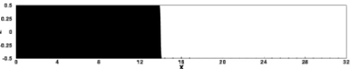
Gravity currents form when a heavier fluid propagates into a lighter one in a predominantly horizontal direction. They are frequently encountered both in the environment and in engineering applications (Huppert, 1986), Simpson, 1997)). Gravity currents can be driven by density differences of the fluids involved, or by differential particle loading. In many situations (a freshwater river flowing into a saltwater ocean, atmospheric flows involving warm and cold air, and many others), the density differences are no more than a few percent, so that the Boussinesq approximation can be employed. However, there are circumstances when the density differences can be much more substantial (industrial gas leaks, tunnel fires, powder snow avalanches, turbidity currents, pyroclastic flows), and the full variable density equations have to be solved. It is desirable to develop simplified models for the prediction of such flows. However, such models are based on a variety of assumptions regarding the nature of the flow whose validity needs to be established first. In this context, high-resolution numerical simulations can be of great value, as they offer access to several quantities that are hard to measure experimentally. The spatially and temporally resolved dissipation field represents one example in this regard. In the following, we will present a brief overview of our numerical simulation results for a variety of gravity currents. We have focused on the lock-exchange configuration, which is the most commonly used geometry for studying gravity currents (see fig. 1).
Basic Equations
The simulations employ a rectangular channel of height H and length L, cf. figure 1. The channel is filled with two miscible fluids initially separated by a membrane. While the left compartment holds a fluid of density ρ1, the right reservoir is filled with a fluid of smaller density ρ2. This initial configuration causes a discontinuity of the hydrostatic pressure across the membrane, which sets up a predominantly horizontal flow once the membrane is removed. The denser fluid moves rightward along the bottom of the channel, while the lighter fluid moves leftward along the top.
The full incompressible Navier-Stokes equations for variable density flows without use of Boussinesq approximation, read
0 . =
∇u 1, (2.1)
( )
S gu ρ µ
ρ = −∇p+∇2
Dt D
. (2.2)
Presented at ETT 2004 – 4th Spring School on Transition and Turbulence September 27th - October 1st, 2004, Porto Alegre, RS, Brazil.
Paper accepted: May, 2005. Technical Editor: Aristeu da Silveira Neto.
Figure 1. Lock exchange configuration. A membrane initially divides the rectangular container into two compartments. The left chamber is filled with fluid of density ρρρρ = ρρρρ1, while the right one contains lighter fluid of
density ρρρρ = ρρρρ2. Upon release of membrane, a dense front moves
rightwards along the lower boundary, while the light front propagates leftward along the upper boundary.
Here
Dt D
denotes the material derivative of a quantity, u = (u,v)T indicates the velocity vector, p the pressure, ρ the density, and
S the rate of strain tensor, while g = geg represents the vector of
gravitational acceleration. In the following, we will keep the kinematic viscosity ν constant for both fluids. In deriving the above continuity equation, it is assumed that the material derivative of the density vanishes, i.e., =0
Dt Dρ
. This common assumption requires small diffusivities of the species concentration. The conservation of species is expressed by the convection-diffusion equation for the concentration c of the heavier fluid. By assuming a density-concentration relationship of the form ρ=ρ2+c
(
ρ1−ρ2)
, we arrive at the following equation for the density fieldρ ρ = ∇2
K Dt D
, (2.3)
where the molecular diffusivity K is taken to be constant. Note that the diffusive term needs to be kept in the above equation in order to avoid the development of discontinuities in the computation of the density field. This holds true even if diffusive effects are very small, as in the case of liquids. In order to nondimensionalize the above set of equations, the channel height H is taken as the length scale, while the density ρ1 the heavier fluid serves as the characteristic density. Velocities are scaled by the buoyancy velocity ub= g′H , in which g’ denotes the reduced gravity (Simpson (1997)), which is related to the dimensional gravitational acceleration g by
( )
γ g gg′= − = 1−
1 2 1
ρ ρ ρ
, where the density ratio is given by
1
1 2 <
= ρ ρ
γ . A characteristic pressure p is given by 2ρ1 b
u . We thus arrive at the following set of governing dimensionless equations
0
= ⋅
( )
Su ρ ρ ρ
γ ρ 2 1 1 ⋅ ∇ + ∇ − − = Re 1 e Dt D
, (2.5)
,
2ρ
ρ = ∇
Pe 1 Dt D
(2.6)
If one were to make use of the Boussinesq assumption, equation (2.5) would instead simplify to
u u
g
2
e −∇ − ∇
= Re 1 p Dt D ρ
. (2.7)
Note that we cannot obtain eq (2.7) from eq (2.5) just by substituting γ = 1, as the hydrostatic pressure field absorbed into the variable p varies between the two cases.
eg is given by the unit vector (sin θ ,0,- cosθ). The three
governing dimensionless parameters in equations (2.4) - (2.6) are the density ratio γ, the Reynolds number Re, and the Péclet number
Pe, respectively, which are defined as
ν
H u Re= b and
K H u Pe= b .
They are related by the Schmidt number
K
Sc=ν , so that
Sc Re
Pe= . . It represents the ratio of kinematic viscosity to molecular diffusivity. For most pairs of gases, the Schmidt number lies within the narrow range between 0.2 and 5. By means of test calculations we established that the influence of Sc variations in this range is quite small, so that in the simulations to be discussed below we employ Sc = 1 throughout. It is to be kept in mind, however, that for liquids such as salt water, Sc≈ 700.
For the purpose of numerical simulations, we recast equations (2.4) - (2.6) into the vorticity-stream function formulation. In this way, the incompressibility condition (2.4) is automatically satisfied throughout the flow field. Let ψ be the streamfunction and ω the vorticity in the spanwise direction. Then the relations
y u z u x v ∂ ∂ = ∂ ∂ − ∂ ∂ = ψ
ω , , and
z v
∂ ∂
= ψ hold, and we obtain
ω ψ −=
∇2 , (2.8)
(
)
DtDv x Dt Du z x Re Dt D ρ ρ ρ ρ ρ γ ρ ω
ω + −
− − ∇ = 1 1 2
(
)(
)
{
x v z u xzvz uz vx xx zz}
Re ρ ρ ρ ρ ρ
ρ ∇ − ∇ + + + −
+ 1 2 2 2 2 4 . (29)
If the dynamic viscosity µ is held constant instead of the ν kinematic viscosity (2.9) takes the form
(
)
DtDv Dt
Du Re
Dt
D x z x
ρ ρ ρ ρ ρ γ ρ ω ρ
ω + −
− − ∇ =
1
1 2 . (2.10)
Computational Approach
The simulations employ equidistant grids in the rectangular computational domain. Spectral Galerkin methods are used in representing the streamwise dependence of the streamfunction and the vorticity fields
(
)
( ) ( )
(
, ,)
ˆ( ) ( )
, , , , ˆ , , x l sin t z t z x w x l sin t z t z x l l l l α ω α ψ ψ ∑ ∑ = = (3.1)where l<N1 /2 and 2π/L. N1 denotes the number of grid points
in the streamwise direction. Vertical derivatives are approximated on the basis of the compact finite difference stencils described by Lele (1992). As in the Boussinesq investigation of Härtel et al. (2000), derivatives of the density field are computed from compact finite differences in both directions. At interior points, sixth order spatially accurate stencils are used, with third and fourth order accurate ones employed at the boundaries. The flow field is advanced in time by means of the third order Runge-Kutta scheme described by Härtel et al. (2000). The material derivatives of the velocity components appearing in the vorticity equation (2.9) are computed by first rewriting them in terms of the local time derivative plus the convective terms. The spatial derivatives appearing in the convective terms are then evaluated in the usual, high order way. The local time derivative is computed by backward extrapolation as follows
(
)
tt n n n ∇ − = ∂ ∂ − / 1 u u u
. (3.2)
This approximation is consistently utilized during the successive Runge-Kutta substeps. Test calculations demonstrated that the low order approximation of this term did not influence the results in a measurable way. The Poisson equation for the streamfunction (2.8) is solved once per time step in Fourier space according to
( )
ˆ +1″−( )
2ˆ +1= ˆm+1 l m l ml lα ψ ω
ψ (3.3)
with the prime denoting differentiation with respect to z.
Boussinesq Gravity Current
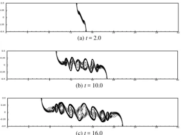
The density difference between two fluids can range from very small to very large. In many geophysical situations such as sea water and fresh water the density difference is very small (within 5%). In cases of small density difference, density variations can be neglected in the inertia term, but retained in buoyancy term where they are multiplied with g. This approximation of the momentum equations is referred to as the Boussinesq approximation. It is accurate for fluids with densities within a few per cent of each other. The formation of a Boussinesq gravity current is shown in fig. 2 for
(a) t = 2.0
(b) t = 10.0
(c) t = 16.0
Figure 2. Concentration contours from a Boussinesq simulation for Re = 4,000, at different times, showing the evolution of a typical Boussinesq gravity .
Non-Boussinesq Gravity Currents
There can be practical situations of interest where the density difference between the two fluids forming the gravity current is larger than a few percent. Turbidity currents and hot gas eruptions from volcanoes are just few examples. In order to study such flows, we cannot use the above Boussinesq approximation. We instead need to solve the complete Navier-Strokes equations involving variable density. For density ratios of For density ratios of γ = 0.92, 0.7, and 0.2, fig. 3 shows contour plots of simulations for Re = 4,000 at time t = 10. Fig. 3(a) still resembles the Boussinesq gravity current, although the symmetry is maintained only approximately. This loss of symmetry can be observed most clearly in the vortex pairing process.
(a) γ = 0.92
(b) γ = 0.7
(c) γ = 0.2
Figure 3. Concentration contours from a non-Boussinesq simulation for
Re = 4,000 at time t = 10 for different density ratios γγγγ, clearly showing the changes in the front speeds and the front heights.
Fig. 3(b) clearly shows that already for γ = 0.7 the dense front moves significantly faster than the light front, and that it has traveled a longer distance than for the γ = 0.92 case. Also the height of the dense front is smaller than that of the light front. These observations can be seen even more clearly in fig. 3(c). We observe
that the Kelvin-Helmholtz instability forms only along the dense front, while the light front is stable. All these observations are in agreement with experimental observations by Ggröbelbauer (1993) and Lowe (2004).
Simplified models of non-Boussinesq gravity currents have been developed by patching an energy-conserving light front to a dissipative dense front via an expansion wave. The validity of this model is confirmed by the dissipation data provided by Birman et al.(2004) The results demonstrate that the dissipation in the light front remains nearly constant as the density ratio changes from 1 to 0.2, while the dissipation level in the dense front increases. This is observed for all values of Re studied.
Gravity Currents on Slopes
Gravity currents in nature and industry frequently flow along slopes. Thus it is important to understand the effects of a sloping bottom on the global properties of gravity currents. Gravity currents along inclines have been modeled in the past using wedge models, cf. Ross et al.(2002}. The wedge shape is used to model the long-term behavior of the gravity current, while it is proposed that in the short term the angle of the slope does not matter. Also it has been noted that friction along the bottom wall does not play an important role in this flow. Thus, in order to better understand the long and short-term behavior of gravity currents on a slope, we present highly resolved numerical simulation results in fig. (4).
Figure 4. Flow for γγγγ = 0.998 at different times for Re = 4,000. The angle of the bottom is 30º to horizontal.
Fig. 4(a) shows that at t = 3 the gravity currents are just beginning to form. There does not appear to be a strong effect of the slope angle during this early phase, as the shape of the currents is similar to the case of a horizontal flow. We observe slight differences in the front propagation velocity, however. Fig. 4(b) shows that soon thereafter much more vigorous mixing takes place along the interface, as compared to the horizontal case. Accelerating fluid layers form behind both fronts, similar to those studied experimentally by Thorpe (1968} in inclined channels. In fig. 4(c) we observe that these accelerated layers, whose dynamics are clearly affected by the angle of the slope, have reached the fronts and start to affect their propagation velocities.
Gravity currents on slopes thus exhibit two different phases: The first phase is characterized by early mixing and the formation of the accelerated fluid layers behind the fronts, while the second phase is dominated by more rapidly advancing gravity current fronts. The simulations give the time for the transition between the two phases
as 9
4
tan −
= φ
φ
t . This is agreement with the results provided by Ross
Particle-Laden Gravity Currents
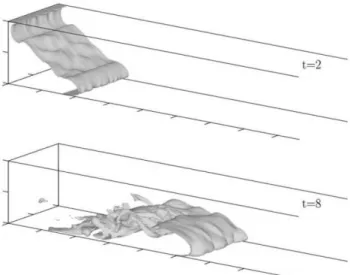
Particle-driven gravity currents form a special class of gravity currents, as their density difference is caused by differential loading with suspended particles (fig. 6). Here we focus on dilute suspensions with volume fractions well below one percent, so that particle-particle interactions can be neglected and coupling between particles and fluid motion is dominated by the transfer of momentum.
Figure 5. The dense front velocity for the gravity current on a slope shown in fig. 4. It can be seen that close to t = 12 there is a jump in velocity of the front. This suggests the transition from the first to the second phase.
Figure 6. Structure of a particle-driven gravity current visualized by isosurfaces of concentration at t = 2 and t = 8. Results are obtained from a three-dimensional simulation for a Grashof number of Gr = 5 x 10⁶ and a
dimensionless settling velocity of us = 0.02 (from Necker et al. (2002b)). In
all cases the concentration value of 0.25 is shown.
The settling of the particles leads to a continued loss of suspended material in the flow. In consequence, at the bottom of the tank a sediment layer forms that grows with time. It has been observed that the sedimentation process is very rapid during the first 10-20 dimensionless time units until about 70% of all particles have settled out. Thereafter, sedimentation slows down substantially. Fig. 7 gives the detailed time history of the sedimentation rate (cf. Necker et al. (2002)). Until t = 14 the sedimentation rate steadily increases. A striking feature of the sedimentation rate is the abrupt change that follows the steady increase, leading to a massive decay of sedimentation rate with time. This change occurs when about half the particles have settled at the bottom, and it coincides with the
time when the front speed of the particle-driven current starts to deviate from the speed of its density-driven counterpart.
Figure 7. Sedimentation rate at the bottom wall of the channel as a function of time. The thin horizontal line indicates the initial value of the sedimentation rate.
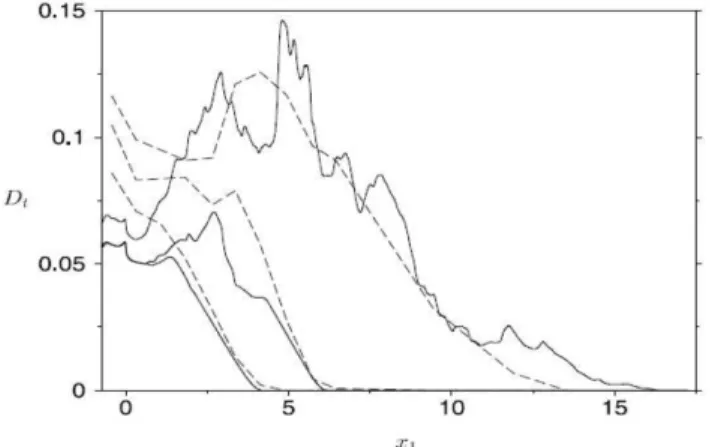
For the sake of direct comparison of computational results with experimental data, we have evaluated the integrated sedimentation profile at the bottom for selected times from a two-dimensional simulation at Gr 108. For this Grashof number, measurements of
Rooji & Dalziel (1998) are available. The small, heavy particles used in the experiments have a non-dimensional settling speed of about 0.02, which is also used in the simulation. In fig. 8 the computational and experimental sedimentation profiles for three different time instants are given in the form of a non-dimensional deposit rate Dt(x,t) per unit span. The curves are normalized such
that the results for the latest time (t→∞), when all particles have already settled out, integrate to unity. Good agreement between the experimental data and the simulation results, which are represented by dashed and solid lines, respectively, is readily seen. Both consistently show the maximum of the final deposition curve to be located some distance downstream of the initial interface location, a feature that was already observed in earlier experiments Bonnecaze
etal. (1993). Differences between experiments and simulations are primarily seen in the region around the initial lock. However, in the experiments this region is presumably affected not only by disturbances induced by the initial stirring of suspension but also by the onset of sedimentation before start of experiment.
Summary
Figure 8. Non-dimensional particle deposit profiles as functions of x. Results for time t = 7.3 and 10.95, and the final profile for (t→→→→∞∞∞∞) after all particles have settled. Solid line: two-dimensional simulation, dashed line: experimental data of Rooji & Dalziel (1998. In both cases Gr = 108, us =
0.02$ (from Necker (2002)).
Acknowledgments
This work has been supported by the National Science Foundation - USA.
References
Benjamin, T. B., 1968, “Gravity currents and related phenomena”, Journal of. Fluid Mechanics, Vol. 31, p.209.
Birman, V. K., Martin, J. E. and Meiburg, E., 2004, “The non-boussinesqlock-exchange problem. Part 2: High resolution simulations”, Journal of Fluid Mechanics (submitted).
Bonnacaze, R., Huppert, H. E. and Lister, J., 1993, “Particle driven gravity currents”, Journal of Fluid Mechanics, Vol. 250, pp. 339-369.
Gröbelbauer, H. P., Fanneløp, T. K. and Britter, R. E., 1993, “The propagation of intrusion fronts of high density ratio”, Journal of Fluid Mechanics, Vol. 250, p. 669.
Härtel, C., Meiburg, E. and Necker, F., 1999, “Vorticity dynamics during the start-up phase of gravity current”s. Il Nuovo Cimento C, Vol. 22, p. 823.
Härtel, C., Meiburg, E. and Necker, F., 1999, “Analysis and direct numerical simulation of the flow at a gravity-current head. Part I: Flow topology and front speed for lip and no-slip boundaries”, Journal of Fluid Mechanics, Vol. 418, p. 189.
Huppert, H. E., 1986, “The intrusion of fluid mechanics into geology”. Journal of Fluid Mech. Vol. 173, p. 557.
Lele, S. K., 1992, “Compact finite differences schemes with spectral-like resolution”, Journal of Comput. Phys., Vol. 103, pp. 16-42.
Lowe, R. J., Rottman, J. W. and Linden, P. F. 2004, “The non Boussinesq lock exchange problem, part I: Theory and experiments”, Journal of Fluid Mechanics (submitted).
Neckar, F., Härtel, C., Kleiser, L. and Meiburg, E, 2002, “High resolution simulations of particle-drivengravity currents”, International Journal of Multiphase Flow, Vol. 28, pp. 279-300.
Rooji, F. D. and Dalziel, S. B., “Time-resolved measurements of the deposition under turbidity currents”. In: Proc. of the Conference on Sediment Transport and Deposition by Particulate Gravity Currents, Leeds, UK.
Ross, A. N., Linden, P. F. and Dalziel, S. B., 2002, “Three-dimensional gravity currents on slopes”, Journal of Fluid Mechanics, Vol. 453, p. 239.
Simpson, J. E., 1997, “Gravity Currents in the Environment and Laboratory”, Cambridge U.P.