Samir Ziada
[email protected] Dept. of Mechanical Engineering McMaster University Hamilton, Ontario L8S 4L7 Canada
Vorticity Shedding and Acoustic
Resonance in Tube Bundles
This paper describes the vorticity shedding excitation in tube bundles and its relation to the acoustic resonance mechanism. These phenomena are investigated by means of velocity and pressure measurements, as well as with the aid of extensive visualization of the unsteady flow structure at the presence and absence of acoustic resonance. Vorticity shedding excitation is shown to be generated by either jet, wake, or shear layer instabilities. The tube layout pattern (in-line or staggered), the spacing ratio, and Reynolds number determine which instability mechanism will prevail, and thereby the relevant Strouhal number for design against vorticity shedding and acoustic resonance excitations. Strouhal number design charts for vortex shedding in tube bundles are presented for a wide range of tube patterns and spacing ratios. Regarding the acoustic resonance mechanism, it is shown that the natural vorticity shedding, which prevails before the onset of resonance, is not always the source exciting acoustic resonance. This is especially the case for in-line tube bundles. Therefore, separate "acoustic" Strouhal number charts must be used when appropriate to design against acoustic resonances. To this end, the most recently developed charts of acoustic Strouhal numbers are provided.
Keywords: Tube bundles, vorticity shedding, acoustic resonance
Introduction
Flow-induced vibrations of heat exchanger tube bundles often cause serious damages resulting in lost revenue and high repair costs. A wide range of flow-induced vibration and noise problems in heat exchangers is reviewed by Païdoussis (1982). The excitation mechanisms causing flow-induced vibrations of tube bundles in cross-flows are generally classified as (a) tube resonance by vorticity shedding, (b) acoustic resonance, (c) turbulent buffeting and (d) fluid-elastic instability. Due to space consideration, this paper will focus only on the first two of these mechanisms for the most common layout patterns of tube bundles. Figure 1 shows these patterns, classified into in-line (IL), parallel triangle (PT), normal triangle (NT), and rotated square (RS) arrays. Note that the normal square (NS) geometry is a special case of the general in-line pattern. As illustrated in Fig. 1, the parallel triangle array has staggered tubes, similar to NT and RS arrays. However, in contrast to the latter arrays, it allows the flow to proceed relatively freely along the lanes between adjacent tube columns, which is somewhat similar to the case of in-line tube pattern. For this reason, as will be shown in this paper, the flow excitations in IL and PT tube bundles display some common features, which are different from those observed in NT
and RS arrays.1
No rmal S qu are (N S) Ro tated Sq u are (R S)
Normal Trian gle (N T) P arallel Tria ngle (P T)
No rmal S qu are (N S) Ro tated Sq u are (R S)
Normal Trian gle (N T) P arallel Tria ngle (P T)
Figure 1. Standard layout patterns of tube arrays and corresponding patterns of flow “lanes” for a selected pitch ratio (P/d = 1.4).
Presented at ETT 2004 – 4th Spring School on Transition and Turbulence September 27th - October 1st, 2004, Porto Alegre, RS, Brazil.
Paper accepted: May, 2005. Technical Editor: Aristeu da Silveira Neto.
Vorticity Shedding and Acoustic Resonance Mechanisms
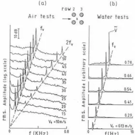
Tube arrays in cross flow are excited, to varying degrees by periodic fluid forces, the frequency of which varies linearly with the flow velocity. This periodic excitation is variously known as: flow periodicity, Strouhal periodicity, or vorticity shedding. It appears in the turbulence and pressure spectra as a narrow band peak, which indicates that it is basically a periodic phenomenon. The turbulence spectra given in Fig. 2 illustrate the dependence of the vorticity
shedding peak (fv) on the gap velocity (Vt). When the frequency of
this vorticity shedding coincides with a mechanical resonance frequency of the tubes, resonant vibration and rapid tube damage can occur, especially in liquid flows. The flow velocity at which this occurs is known as the critical flow velocity for tube resonance, and the velocity range over which the tubes exhibit large amplitude vibration is referred to as the "Lock-in" range. Although this excitation has been recognized since the 1950's, its cause has been disputed in the literature (Owen, 1965). Recent studies have shown clearly that it results from vortex shedding from the tubes (Weaver, 1993; Ziada et al., 1989a & 1992).
Acoustic modes of the tube bundle containers can also be excited by gas flow across the tubes. The excited modes are those consisting of acoustic standing waves in a direction normal to the tube axes and the flow direction, see Fig. 3. At resonance, an intense pure tone noise, which can reach 175 dB, is produced. This level is sufficiently high to disturb the operation of power plants and cause structural failure. The excitation mechanism of these resonances is strongly dependent on the tube layout pattern and spacing ratio.
Figure 3. Schematic presentation of the wind tunnel test section illustrating the distributions of acoustic pressure associated with the first and second acoustic modes. P(f1 ): pressure distribution of first acoustic mode; P(f2): second mode.
In this paper, normal triangle and rotated square patterns will be discussed first because their flow characteristics have some similarities. Attention will then be focused on the in-line geometry, which exhibits unsteady flow features distinctively different from those observed for normal triangle arrays. The parallel triangle array is discussed last because it is more complex as its geometry combines features from the in-line and the normal triangle patterns. In general, the investigated bundles will be classified into small, medium and large tube spacings. The details of the experimental techniques used in this study can be found in Ziada & Oengoeren (1992, 1993, 2000) and Oengoeren & Ziada (1992a, 1992b, 1998).
Normal Triangle Tube Arrays
Overview of Flow Periodicity
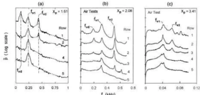
Typical pressure spectra for three normal triangle arrays with a
small, an intermediate, and a large pitch ratio, Xp = P/d = 1.6, 2.08
and 3.41, respectively, are given in Fig. 4. For each case, spectra of rows 1-5 taken during air tests are illustrated. Three frequency
components are observed at the first row for the cases Xp = 1.6 and
2.08 and two components are apparent in the case of Xp = 3.41.
These components are referred to hereafter as fv2, fvl and fvd, from the
highest to the lowest, respectively.
As observed in Fig. 4(a), the small spacing ratio, the
components fvd and fvl have relatively broader frequency bands as
compared with the peak fv2. The peak fvd becomes hardly discernible
at the second row. The peak fv2 also weakens substantially at the
inner rows and totally disappears at row 4. Only the fvl component is
sustained at rows 1 to 5. It should be mentioned at this point that the
spectra for this case (Xp = 1.6) were measured with a microphone
located on the top wall of the test-section. Therefore, the responses of the first and the second acoustic modes were also present in addition to the vortex-shedding peaks. These acoustic responses were removed from these spectra and replaced by dotted lines to avoid a possible confusion. The pressure spectra of the intermediate spacing case, Fig. 4(b), were measured by means of a microphone connected to a pressure tap on the tube. They show similar
characteristics as the small spacing case; however, the peak fv2 is
stronger and is sustained somewhat deeper inside the array up to the fourth row. The pressure spectra of the large spacing array, Fig.
4(c), contain only two components, fv1 and fv2, at the first row. In
contrast to the previous two cases, both components are rather broad-banded, even at the front rows. However, the development of these peaks towards the inner rows is similar to the other cases.
The frequency component fvd appears to be broad-banded and
tends to disappear as one of the other peaks becomes weaker. In fact, a close look at the spectra of the intermediate spacing array
shows that fvd is exactly equal to the difference between fv2 and fv1
(fvd = fv2 - fv1). These features suggest that the component fvd results
from nonlinear interaction between fv1 and fv2. This phenomenon of
nonlinear interaction between different frequency components in separated flows has been reported by many researchers; see, for
example, Miksad (1973). The fvd component was studied carefully in
all cases tested and it was verified that it stems from the interaction
between the two components fv1 and fv2, and not from another
periodic flow structure.
The results presented in the foregoing illustrate that the flow activities in the three arrays exhibit some similarities. However, it should also be emphasized that these results are based on some rather selective data. These data were obtained utilizing different measurement techniques as well as different Reynolds numbers. An examination of the data provided in the literature for similar geometries shows that some of the features mentioned above have been overlooked because of differences in the test conditions, measurement techniques and/or the location of measurements. In order to establish a baseline for all geometries, the tests of each of the above arrays were performed according to a standard procedure (Oengoeren & Ziada, 1998). The objective was to study the effects of Reynolds number and row depth on the vortex-shedding process. These issues are discussed next for intermediate tube spacings and then briefly for small and large spacing ratios.
Figure 4. Typical pressure spectra measured at rows 1 to 5 and (a) on top wall of the wind tunnel, (b) and (c) on the tubes of normal triangle arrays in air flow. (a) Xp=1.61, R=49600; (b) Xp=2.08, R=26300; and (c) Xp=3.41, R=6000.
Normal Triangle Arrays with Intermediate Tube Spacing
Effect of Reynolds Number
The spectra of pressure fluctuations on a tube in the second row and those of the velocity fluctuations detected by a hot-film located behind rows 1 to 5 are given in Fig. 5. These results cover a Reynolds number range of 17300-52000. Only one vortex-shedding
peak, fv2, is observed at low Reynolds numbers (Re < 22200). It
corresponds to a Strouhal number of 0.4. As the Reynolds number is increased to 22200, this peak becomes weaker and a second peak, fv1, appears in the spectrum with a Strouhal number of 0.26. The
peak fv1 is rather weak and broad-banded at this Reynolds number.
fv1 and the weakening of fv2 components continue. At a Reynolds
number of 32000, the amplitude of fv1 becomes significantly
stronger than fv2. As this process of frequency change continues, a
third peak, fvd = fv2 - fv1, corresponding to a Strouhal number of 0.14
emerges in the pressure spectra for Reynolds numbers over 22200. It
is interesting to note that the difference component fvd reaches its
strongest level at the second row and when both components fv1 and
fv2 are relatively strong. The frequency modulation behind row 2 vanishes when the Reynolds number is increased above 45000, where the vortex shedding transforms into a single-frequency event
at the lower-frequency component fv1 (S = 0.26). A typical pressure
spectrum in this range is given in Fig. 5(a) for Re = 52000. Similar pressure and hot-film measurements carried out on the first row showed that the same transformation also occurs behind this row. This means that the vortex shedding phenomenon becomes a single-frequency event with a Strouhal number of 0.26 throughout the whole bundle in the high Reynolds number range.
V e lo c it y f lu c tu at io n P re ss u re f lu c tu at io n , P a Strouhal number Row 2 Re=52000 32000 22200 17300
(a) Air tests (b) Water tests
Re=34800 V e lo c it y f lu c tu at io n P re ss u re f lu c tu at io n , P a Strouhal number V e lo c it y f lu c tu at io n P re ss u re f lu c tu at io n , P a Strouhal number Row 2 Re=52000 32000 22200 17300
(a) Air tests (b) Water tests
Re=34800
Figure 5. Spectra of (a) pressure fluctuations measured on a tube in the second row for different Reynolds numbers and (b) velocity fluctuations measured by a hot-film behind rows 1 to 5 of a normal triangle array with intermediate spacing ratio Xp= 2.08.
Effect of Row Number
Figure 5(b) shows the effect of row number at Re of 34800. Additionally, pressure spectra measured on the first five rows were previously presented in Fig. 4(b). As observed in these figures, the
vortex shedding peaks fv1 and fv2 and the associated difference
component fvd exist in both pressure and velocity spectra in the front
rows. The component fv2 becomes gradually weaker in the
downstream direction and ceases to exist rather promptly after the
third or fourth row. In contrast to fv2, the component fv1 exists in the
spectra for the whole bundle at this particular Reynolds number range and becomes the only peak existing after the fourth row.
From the foregoing results, it may be suggested that data obtained in tube bundles having less than five rows may not be representative. At relatively low Reynolds numbers, the changes in the vortex-shedding behavior might be displayed only partly in the results. On the other hand, measurements made solely on rows deeper than the fourth row may not reflect all aspects of vortex shedding, either. In such cases, the multiple frequency nature of vortex shedding and its transformation to a single-frequency event may be overlooked.
Nature of Vorticity Shedding
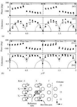
In order to investigate the local and global characteristics of the vortex-shedding process that dominates over the whole bundle, the phase and the coherence distributions of the fluctuation velocity
behind several rows were measured in detail as functions of the
vertical distance, y. A diagram showing the measurement locations
is given at the bottom of Fig. 6. A length of two vertical pitches was traversed behind rows 3, 5, 7 and 9 in order to reveal the relation between the flow patterns in different columns and rows and to capture the overall spatial pattern of flow structure.
As shown in Fig. 6, the fluctuating pressure signal detected by means of a pressure tap located at the mid-span of a tube in the fifth row was used as a reference in all the coherence and phase measurements of the velocity fluctuations. The phase of the velocity
fluctuations at the frequency component fv1 measured behind rows 3,
5 and 7 for a velocity of 21.2 m/s (Re = 25500), are plotted in Fig.
6(a1). The positions y/P = 0, 1 and 2 correspond to the centerlines of
the tube wakes. All the phase data of fv1 belonging to different rows
produce a single distribution as observed in this figure. This means that the flow structures behind the three rows are identical and synchronized (because the associated phase distributions are similar and are also in phase with each other). Moreover, the data belonging to neighboring tube wakes (or flow lanes) have identical distributions, e.g. the phase distribution in flow lane 11 is identical to that in flow lane 12. This indicates that the flow pattern is identical and synchronized in the wakes of neighboring tubes in each row. These rather remarkable features illustrate the fact that the flow patterns in the wakes of all tubes in rows 3, 5 and 7 are identical and synchronized. This flow pattern is identified as alternating vortex shedding from the tubes when the phase in each tube wake is examined (a phase jump of 180º occurs at the center of each wake).
The coherence distributions associated with the above phase distributions are given in Fig. 6(a2). The distributions belonging to all rows are similar. The coherence drops to a minimum at the centers of the tube wakes and the flow lanes, where a phase jump occurs because the vortices at the opposite sides of these locations have opposite circulations, see the diagram at the bottom of Fig. 6.
Figure 6. Distributions of phase and coherence of velocity fluctuations at
fvlfor velocities of (a) 21.2 m/s (Re = 25500) and (b) 33 m/s (Re = 39600) behind rows 3, 5, 7 and 9. The pressure fluctuation on a tube located in the fifth row was taken as the reference signal for all measurements. Air tests: ○
, row 3; ● , row 5;
◊
The coherence increases rapidly away from these locations, because the velocity fluctuations become better defined, and it reaches a maximum of 0.75. A high coherence between the velocity fluctuations at different locations indicates that these fluctuations are associated with the same (global) flow phenomenon. The phase and coherence measurements were repeated for rows 5, 7 and 9 at a higher velocity of 33 m/s (Re = 39600) in order to verify this very
organized flow behavior. The results are given in Fig.6(b). All the
characteristics of the previous low Re case are evident also in this case, indicating that the same flow structure exists at high Reynolds numbers. Additionally, a significant enhancement is observed in the coherence level at this velocity, reaching a maximum of 0.98 in comparison with a level of 0.75 in the low velocity case. Both cases are clearly away from the range of acoustic resonance (Oengoeren & Ziada, 1998). Thus, this globally organized flow cannot be attributed to a coupling with acoustic standing waves, but rather to a fluid dynamic mechanism that gains in strength as the Reynolds number is increased. The impingement of the shed vortices on the downstream cylinders may well be the source of the fluid dynamic mechanism that enhances this global mode of vortex shedding (Rockwell & Naudascher, 1979).
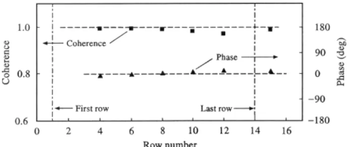
Figure 7. Distributions of coherence and phase of vortex-shedding component fvl as functions of row depth at a velocity of 22 m/s (Re =
26400). The signal of row 2 was taken as the reference signal for all other rows.
Finally, Fig. 7 shows the coherence and the phase difference between the second and the deeper rows for the vortex shedding component fv1. These results were obtained by means of two microphones located on the top wall of the test-section. It is seen that the vortices shedding from all rows are correlated and are in phase with each other implying a total synchronization of vortex shedding in the bundle.
Flow Visualization
The flow visualization study was carried out in the water channel. First, the frequency of vortex shedding was measured when the free surface in the test-section was covered, thereby precluding the formation of free-surface waves. The results of Strouhal number obtained by means of a hot film located at different rows were found to be similar to those obtained from the air tests (for more details see Oengoeren & Ziada, 1998).
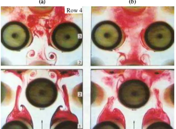
A series of typical visualization photographs are given in Fig. 8, showing the flow structure behind the first two rows in a Reynolds number range of 1000 < Re < 7000. Alternating vortices are shed from the tubes of the first row. They then proceed into the flow lanes of the second row and promote vortex formation from the tubes of this row. The same flow pattern is observed in all the photographs despite the large range in Reynolds number. Symmetry is observed in the vortex-shedding pattern with respect to the center of the tubes in the second row. Although this symmetric pattern occurs only intermittently, it was much more persistent than the antisymmetric one which was occasionally observed.
The above results suggest that vortex shedding from the first and the second rows occurs at the same frequency, which is the
high-frequency component fv2. This was confirmed by counting the
frequency on the video monitor.
(a)
(d) (c)
(b) row (a)
(d) (c)
(b) row
Figure 8. Flow structure behind the first two rows of an intermediate spacing normal triangle tube bundle (Xp = 2.08; d = 25 mm) in water for Reynolds numbers of (a) 1000, (b) 1800, (c) 5000, and (d) 7000.
Vg Vg
Figure 9. Alternating vortex shedding behind row 3 of a normal triangle array. Xp = 2.08; d=60mm; Re= 35500.
In order to show the vortex shedding pattern at high Reynolds numbers, where a single- frequency vortex shedding phenomenon occurs, the flow was visualized inside an array of larger diameter tubes. With this arrangement, the visualization of the flow at a Reynolds number of 35500 was possible. As shown in Fig. 9, a persistent alternating vortex shedding was observed behind the third row. Most importantly, counting of these vortices on the video has
shown that they correspond to the frequency component fv1, which is
in agreement with the hot-film spectra measured behind this row. A
pattern belonging to fv2 component has not been observed in the
flow visualization photographs taken behind this row at this Reynolds number.
Normal Triangle Arrays with Large Tube Spacing
Effect of Reynolds Number
The effect of Reynolds number on vortex shedding in a widely
spaced normal triangle array (Xp = 3.41) is illustrated in Fig. 10.
Typical spectra of the velocity fluctuations behind the second row measured in airflow are given in Fig. 10(a). The two frequency
components appearing in these spectra correspond to fvl and fv2,
according to the definitions of these components in Fig 4. There are three Reynolds number ranges where different vortex shedding characteristics are observed. At low Reynolds numbers, Re < 6600,
both fvl and fv2 exist and follow the Strouhal number lines 0.2 and
0.28, respectively. In this range, the fv2 is significantly weaker and
> 18200, only the vortex-shedding component fvl remains in the spectra. In fact, this component becomes narrower and stronger as the Reynolds number is further increased. The spectra belonging to the range of 6600 < Re < 18200, show that vortex shedding changes from a multi-frequency to a single-frequency phenomenon. Within
this transition range, the vortex-shedding component fv2 is gradually
shifted towards the component fvl as the Reynolds number is
increased. The transition is completed as fv2 unites with fvl. To
illustrate this process better, the Strouhal numbers of both components are plotted as functions of the Reynolds number in Fig.
10(b), including both the air-and water-test data. The shift of fv2
towards fvl is depicted clearly in this plot. Although the flow velocity
in the air tests is about two orders of magnitude higher than that in the water tests, the transition range in both cases occurs at the same Reynolds number.
fv1
fv2
(a) (b)
fv1
fv2
(a) (b)
Figure 10. Transition of frequency components in a normal triangle array with large spacing (Xp=3.41). (a) Velocity spectra measured behind the second row in air, and (b) Strouhal number of vortex shedding measured in air and in water. Triangle data: Air tests; circular: water tests.
row
2
1 3
row
2
1 3
Figure 11. Typical flow patterns behind the first two rows of a large spacing normal triangle array for Re = 4800; Xp = 3.41, d = 16mm.
Flow Visualization
Figure 11 shows flow structures behind for the large spacing array at Re = 4800. Well-defined alternating vortices are shed from almost every tube of front rows. At this Reynolds number, the dominance of an antisymmetric mode of flow pattern is evident. The frequency of vortex shedding from the first two rows was counted from the video monitor. Vortex shedding from the first row occurred
at the high-frequency component fv2, but that from the second row
occurred at the low-frequency component fv1. Weaver et al. (1993)
reported similar observations for rotated square arrays.
The air-test results of this large spacing array have shown that a single-frequency vortex shedding sets in at Reynolds numbers higher than approximately 12000. This was confirmed by a flow visualization study in an array with larger diameter tubes, which allowed the Reynolds number to be increased above 12000 (Oengoeren & Ziada, 1998).
Normal Triangle Arrays with Small Tube Spacing
Nature of Vorticity Shedding
Typical spectra of pressure fluctuation on rows 1-4 of a small
spacing normal triangle array (Xp=1.61) are given in Fig. 12. A
narrow-band peak at a Strouhal number of approximately 0.6 is clearly seen in the spectra. This Strouhal number, which
corresponds to the vortex-shedding component fv2, is similar to that
measured for the same geometry by Zukauskas & Katinas (1980). The background turbulence level increases gradually as the flow progresses into the bundle; however, no other distinct peaks that can be attributed to periodic flow activities can be seen in these spectra. A broadband peak can be seen at a Strouhal number of about 0.15. Despite its broadband nature, this peak does not seem to be generated by the turbulent buffeting mechanism because it exists at the second row only and within a certain range of Reynolds number. The pressure spectra given in Fig. 12 seem to be somewhat different from those presented in Fig. 4(a), which displays a
better-defined low-frequency component, fvl. It should be recalled that the
results of Fig. 4(a) were obtained by means of a microphone on the top wall of test section. This microphone senses the integrated effect of the pressure fluctuations over the area of the sensing element, which is substantially larger than the pressure taps on the tubes. The
enhancement of the peak at fvl in the microphone signal is therefore
attributed to an improved coherence and correlation length of the pressure fluctuation at this frequency. Undoubtedly, the
low-frequency component fvl becomes weaker, broader and develops at
higher Reynolds number in this small spacing array. It seems to be associated with the development of the flow turbulence at the downstream rows.
Strouhal number Strouhal number
Flow Structure
Figure 13(a) displays the flow structure behind the first three rows at Reynolds number of 3050. Well-defined but relatively weak vortices are shed behind the first row. They become rather strong behind the second row despite their relatively small scale. However, they are diffused at the third row, and vortex-like structures totally disappear downstream of this row. As in the case of intermediate spacing, alternating vortex shedding occurs behind the first row and symmetric vortices are shed from the second row. This pattern does not seem to be intermittent in this array, as opposed to the observations of the intermediate and the large spacing arrays. The flow structure was observed to remain the same when the Reynolds number was increased up to 15250, Fig. 13(b). The video counting of the frequency of vortex shedding from rows 1 and 2 verified that
they are fv2 vortices and correspond to the Strouhal number S2 =
0.55.
(a) (b)
Row 4
(a) (b)
Row 4
Figure 13. Typical flow patterns behind rows 1-3 for Reynolds numbers of (a) Re = 3050 and (b) Re = 15250 in a small spacing normal triangle array. Xp = 1.61, d = 60mm.
Acoustic Resonance of Normal Triangle Arrays
Since the vortex-shedding frequency increases linearly with the flow velocity, it may coincide with the frequency of an acoustic mode. Near the condition of frequency coincidence, powerful acoustic resonances may be produced. The acoustic modes of interest are those consisting of standing waves in a direction normal to the flow and the tube axis. As shown in Fig. 3, the first acoustic
mode, fa1, consists of half a wavelength (λ/2) and the second, fa2,
constitutes a full wavelength (λ) between the top and the bottom walls of the wind tunnel.
A typical example for normal triangle arrays is illustrated in Fig. 14, which shows the acoustic response of a large spacing array with Xp=3.41. An acoustic resonance is initiated as the vortex-shedding
frequency fv1 coincides with the first acoustic mode frequency, fa1, at
a velocity of 42 m/s. A lock-in of the vortex- shedding frequency with the acoustic resonance frequency occurs in the velocity range of 42-51 m/s. Within this range, the SPL increases rapidly until it reaches a level of 156dB.
Figure 14. Sound pressure level (SPL) of the vortex shedding component fv1 and the first acoustic resonance mode fa1, and the corresponding
frequency distributions as functions of gap velocity Vg in a large spacing
normal triangle array.
It should be noted that in this particular case of large spacing,
the higher vorticity shedding component, fv2, did not excite the
acoustic resonance. The ability of this component to excite acoustic resonance increases substantially as the tube spacing ratio is
decreased. In fact, for the other tube spacings discussed above, Xp =
1.61 and 2.08, the acoustic modes were excited by the vortex
shedding component fv2 (for further details see Oengoeren and
Ziada, 1998). For this reason, design against acoustic resonance should be based on the fact that both vorticity components are capable of causing acoustic resonance.
Strouhal Numbers of Normal Triangle Arrays
The Strouhal numbers of the main components of vortex shedding in normal triangle arrays are given in Fig. 15. A particular criterion was not set in the selection of the data points and, therefore, some of them may not be reliable because they were extracted from either tube or acoustic resonances. However, the
results of the three arrays discussed above indicate that the Strouhal
numbers at the onset of acoustic resonances in normal triangle arrays approximate those of the natural vortex shedding away from resonance conditions. Thus, the use of these data to construct a chart of Strouhal numbers for normal triangle arrays seems to be justified.
For the sake of clarity, the non-linear interaction component fvd is
not included in the Strouhal number chart. This is because this component does not seem to cause any "harmful effects", at least within the tested ranges of spacing ratios and Reynolds numbers. The Strouhal number given in Fig. 15 is defined as:
S = fv d/Vg (1)
where fv is the shedding frequency, d is the tube diameter and Vg is
the gap flow velocity.
As expected, the data gather around two Strouhal number lines,
S1 and S2. The points on the line S2 correspond to the vortex
shedding fv2 observed mainly behind the front rows. However, at
high Reynolds numbers, this component may totally disappear in
bundles with intermediate and large spacing ratios (Xp > 2).
S
tr
o
u
h
al
n
u
m
b
er
Spacing ratio, Xp
S
tr
o
u
h
al
n
u
m
b
er
Spacing ratio, Xp
Figure 15. Strouhal number data of vorticity shedding components in normal triangle arrays as function of the spacing ratio. Refer to Oengören & Ziada (1998) for data sources.
The line S1 belongs to the frequency component fv1. This
component has the characteristics of turbulent buffeting excitation
for small tube spacings (Xp ~ 1.6); however, it is associated with
well-defined vortex shedding at the inner rows for larger tube
spacings (Xp > 2). Moreover, it becomes the only flow periodicity
existing in bundles with large spacing ratios and at high Reynolds numbers. The Reynolds number range for which this component becomes dominant depends on the particular spacing ratio.
Whether acoustic resonances are excited by fv1, fv2 or both
depends on the spacing ratio. For spacing ratios of less than about 1.7, acoustic resonances are liable to the high-frequency
component, fv2. The lower modes, however, may not be excited
because the frequency coincidence occurs at low dynamic heads where the vorticity shedding excitation may still be weak in comparison to the system acoustic damping. Several acoustic damping criteria have been developed by Chen (1968), Fitzpatrick (1986), Ziada et at. (1989b), Blevins & Bressler (1992) and Eisinger et at. (1992).
For intermediate spacings, 1.8<Xp<2.7, either frequency can
excite acoustic resonances. However, those excited by the high-frequency component are generally weak, whereas those excited by the lower component are very strong and can be destructive. Other researchers (e.g. Blevins & Bressler, 1987a, b) also suggested that the higher component excites the lower modes only weakly, if at all.
At high Reynolds numbers, the low component fv1 becomes the only
relevant excitation anyway.
Acoustic resonances of large spacing arrays, Xp > 2.8, are
excited by the lower-frequency component only. Since the higher component exists only at low Reynolds numbers and appears only at the first row or two, the fluctuating energy associated with it is presumably too small to excite resonances.
The boundaries between small, intermediate and large spacing ratios are obviously not as well defined as might be suggested by the above. Those boundaries suggested above are based on the results of a limited number of experiments. Additional tests of geometries within the transitional regions are needed.
An important feature of normal triangle arrays is that acoustic resonances are excited by the vorticity-shedding excitation that dominates before the onset of resonance. This implies that the Strouhal number charts of vorticity shedding can be used to design against acoustic resonances. In order to provide a better prediction
means of Strouhal number, empirical forms of S1 and S2 have been
obtained from the least-squares approximation of the data points in Fig. 15 and are given by the formulae:
) 1 p X ( 62 .
3 0.45
1 1
S
−
= ,
) 1 p X ( 4 .
2 0.41
1 2
S
−
= (2)
Rotated Square Tube Arrays
The main flow characteristics of rotated square arrays are similar to those of normal triangle arrays, which are discussed in detail in the previous section. For this reason, only the Strouhal number chart is given here, see Weaver et al. (1993) for details.
Rotated square arrays Rotated square arrays
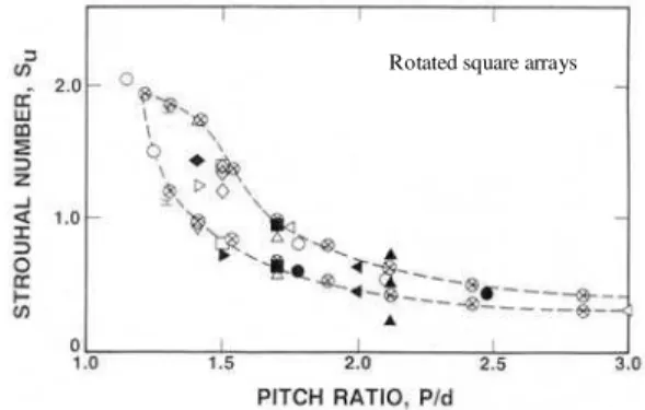
Figure 16. Strouhal number chart for rotated square arrays. The Strouhal number is based on the upstream velocity, Weaver et al. (1993).
Figure 16 depicts the Strouhal number of vorticity shedding as a
function of the pitch ratio Xp. It is important to recognize that this
Strouhal number Su is based on the upstream flow velocity:
Su = fv d/Vu (3)
where , fv is the vortex shedding frequency, d is the tube diameter,
and Vu is the upstream flow velocity. The data points in Fig. 16 are seen to collapse on two Strouhal number lines. The higher corresponds to vortex shedding from the front rows, and the lower is caused by vortex shedding from the inner rows. As expected, the Strouhal number decreases when the pitch ratio is increased.
Previous studies indicate that acoustic and tube resonances can be excited by either of the Strouhal numbers presented in Fig. 16. It is therefore recommended to use Fig. 16 for design purposes in order to assess the possibility of acoustic or tube resonance.
In-Line Tube Arrays
In-Line Arrays with Intermediate Tube Spacing
An array with intermediate spacing ratios (XL/XT = 1.75/2.25) is
studied in air and water flows. Attention is focussed on the first five rows, within which the vorticity shedding excitation is fully developed. Figure 2 shows typical velocity spectra for air and water tests of this array. The velocity fluctuations are seen to occur at a
well-defined (single) frequency, fv, which follows a Strouhal number
of S = fv d/Vt = 0.15, where Vt is the gap velocity, i.e. the same as
Vg. In the air tests, a higher harmonic component at the frequency
2fv is also present due to nonlinear effects of flow instability as discussed by Ziada & Rockwell, 1982.
Effect of Reynolds Number
The effect of the flow velocity on the rms amplitude of the
fluctuating velocity, v, is shown in Fig. 17 for the water tests. The
increased, the rms amplitude of the fluctuating velocity is seen to
increase until it reaches a saturation value ≈ 12% of the gap
velocity. This saturation of v/Vt occurs when the spatially growing
flow instability reaches its fully developed phase (see e.g. Sato, 1960; Freymuth, 1966; and Miksad, 1972). It is important to point
out that increasing the flow velocity causes the ratio v/Vt, and not
only v, to increase. Since the ratio v/Vt, at a fixed position,
represents the degree of development of the flow instability, the results of Fig. 17 indicate that the flow instability behind a certain row becomes more developed as the flow velocity (or the Reynolds
number) is increased. This implies that the position at which the
flow instability becomes fully developed moves upstream as the Reynolds number is increased.
Vt (m/s)
v/
V
t
(%
)
Vt (m/s)
v/
V
t
(%
)
Vt (m/s)
v/
V
t
(%
)
Figure 17. Dimensionless amplitude of fluctuating velocity vbehind row 4 in water tests. XL= 1.75; XT = 2.25.
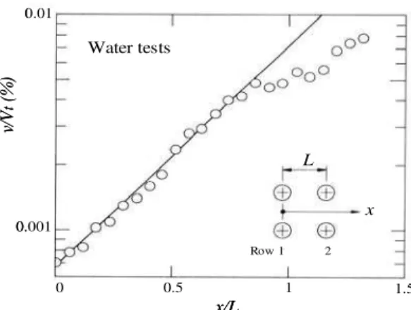
Streamwise Development of Vorticity Shedding
The streamwise development of the flow was measured during the water tests. As shown in Fig. 18, the amplitude increases in the downstream direction and reaches saturation near the fifth row, about 13%. Behind each row, the fluctuating velocity grows rapidly, but this rapid growth is impeded by the presence of the tubes of the
subsequent rows, resulting in the amplitude plateaux at x/L = 1, 2
and 3. These plateaux make the evaluation of the disturbance growth rate rather difficult. Detailed measurements were therefore carried out between the first two rows to gain more insight into the initial stage of the disturbance growth. As shown in Fig. 19, the fluctuating velocity grows exponentially in the downstream direction before it is hindered by the tubes of the second row. This exponential growth accords with the prediction of the hydrodynamic stability theory for separated flows, i.e. shear layers, jets and wakes (Michalke 1965; Bajaj & Garg 1977).
x/L
Row Number
v/
V
t
(%
)
Water tests
x/L
Row Number
v/
V
t
(%
)
Water tests
Figure 18. Development of the velocity fluctuation along a centerline of a flow lane. Water tests; Re = 6.8x10³
.
x/L
v/
V
t
(%
)
Water tests
Row 1 2
0 0.5 1 1.5
0.001 0.01
x L
x/L
v/
V
t
(%
)
Water tests
Row 1 2
0 0.5 1 1.5
0.001 0.01
x L
Figure 19. Initial exponential growth of the velocity fluctuation. Water tests; Re = 6.8x10³.
The air test facility was used to measure the distributions of the fluctuating velocity amplitude within the development region of the flow instability. The measurements were carried out along the lines centred between the tube rows, and at a flow velocity of 30.6 m/s (Re = 3.8 x 10⁴). Figure 20 depicts the distributions across the sixth and the seventh flow lanes (hereafter referred to as jets). The distributions across the fourth and fifth jets were also measured and were found to be similar to those given in Fig. 20. As shown in this Figure, the velocity fluctuations behind the first row are much stronger at the edges of the jet than in its core. This distribution indicates that the flow instability is initiated by the inducement of small velocity perturbations into the shear layers, which separate from the tubes of the first row. These velocity perturbations are amplified exponentially in the downstream direction, as has been shown already in Fig. 19. Because the Reynolds number is relatively high, the fluctuation amplitude reaches 13% of the gap velocity already behind the second row. Interestingly, the fluctuation amplitude in the middle of the jet becomes comparable to that at the jet edges. Further downstream, behind the fourth row, the fluctuation amplitude in the middle of the jet becomes substantially higher than that at the jet edges. This gradual change in the shape of the amplitude distributions will be discussed later in conjunction with the phase measurements and the flow visualization study.
v/Vt(%) y/T
Behind row 2
x= 3L/2
Behind row 4
x = 7L/2 Row 1
x= L/2
Je
t
7
Je
t
6
v/Vt(%) y/T
Behind row 2
x= 3L/2
Behind row 4
x = 7L/2 Row 1
x= L/2
Je
t
7
Je
t
6
Figure 20. Distributions of the dimensionless velocity fluctuation behind the first, the second and the fourth rows. Air tests, Re = 3.8x10⁴
|y -y 4 |/ T |y -y 6 |/ T Je ts 6 + 7 Je ts 4 + 5 Je ts 5 o r 7 Je ts 4 o r 6
φ
vφ
va b c Ŷ /T Ŷ = O y-y3 ∆ y-y5 |y -y 4 |/ T |y -y 6 |/ T Je ts 6 + 7 Je ts 4 + 5 Je ts 5 o r 7 Je ts 4 o r 6
φ
vφ
va b c |y -y 4 |/ T |y -y 6 |/ T Je ts 6 + 7 Je ts 4 + 5 Je ts 5 o r 7 Je ts 4 o r 6
φ
vφ
v|y -y 4 |/ T |y -y 6 |/ T Je ts 6 + 7 Je ts 4 + 5 Je ts 5 o r 7 Je ts 4 o r 6
φ
vφ
va b c Ŷ /T Ŷ = O y-y3 ∆ y-y5
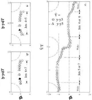
Figure 21. Phase distributions of the velocity fluctuation behind the fourth row at x = 7L/2. Air tests, Re = 3.8 x 10⁴
. (a) ○ , φv4;∆, φv5 + π ; (b) ○ ,
φv6;∆, φv7 + π ; (c) ○ , φv4 and φv5 ;∆, φv6 and φv7; ● , ▲ ,reference
locations.
Phase Relations
The phase distribution of the velocity fluctuation behind the
fourth row is given in Fig. 21.The round data points in insets a & b
represent the phase variations across jets 4 and 6, respectively. The triangular data points correspond to the phase across jets 5 and 7, but after adding a value of π. The phase distribution across anyone jet is seen to be symmetric, i.e. the velocity fluctuations occurring at one edge of a jet is in phase with that at the other edge. Moreover, the velocity fluctuation in any jet as a whole is 180° out of phase with that in the neighboring jet. The phase distributions across the four jets 4 to 7 are presented together in Fig. 21(c). This figure emphasizes the remarkably organized nature of the flow activities. Jet 5, for example, is in phase with jet 7, but is 180° out of phase with the neighboring jets (jets 4 and 6). Additional measurements behind other rows yielded similar results.
Global Structure of Vorticity Shedding
Flow visualization pictures taken at different locations within the array, but at the same time instant of the cycle, were pieced together to construct the development of the flow structure within the first five rows. As shown in Fig. 22. The flow structure in the flow lane, Fig. (a), displays, very clearly, a symmetric mode of an unstable jet. The symmetry with respect to the jet centerline and the clarity of the jet structure are rather remarkable. In the tube wakes, Fig. (b), the vortices form in an anti-symmetric pattern. Moreover, the vortex pattern in each wake is nearly out of phase with those in the upstream and downstream wakes. It should be mentioned here that this anti-symmetric pattern in the tube wakes is phenomenologically different from the alternating vortex shedding in the wakes of isolated cylinders.
Row (a) (b) 1 5 4 3 2 Row (a) (b) 1 5 4 3 2
Figure 22. Flow visualization photographs showing the global flow structure in (a) a flow lane and (b) several tube wakes. Re = 1.5x10⁴.
Figure 23. Overview of the resonant flow structure in the array at the same instant of time in a period of surface wave resonance.
Description of Flow Instability in In-Line Arrays
undergoes a spatial exponential growth, which is in accordance with the linear theory of hydrodynamic stability. Furthermore, the amplitude and the phase of the initial velocity fluctuation have symmetric distributions with respect to the jet centerline. These initial distributions dictate the symmetric pattern of the jet instability developing downstream. The interaction of the developed jet with the downstream tubes is fed back upstream, where new perturbations are induced at the initial region near separation.
The jet instability occurs at a preferred symmetric mode. Large-scale vortices are formed symmetrically at both sides of each flow lane. Because of the kinematic constraints imposed by the large size of the formed vortices and the associated mass transfer across the wakes, vortices are forced to form anti-symmetrically in the tube wakes. This dictates the phase difference between the flow activities in adjacent flow lanes. Thus, the jet instability occurring in each flow lane is 180° out of phase with that occurring in the neighboring lanes.
Simulation of Resonance by Means of Surface Waves in Water Channel
The acoustic resonance was simulated by a transverse surface-wave resonance in the water channel. During the water tests on the intermediated spacing case, the first mode of the transverse standing waves was excited. This mode consisted of a half wavelength spanning the width of the channel. Since the tubes were mounted vertically in the channel, the particle velocity of the surface wave, away from the sidewalls, had a predominant component in a direction normal to the flow and the tube axes. Moreover, the standing wave was found to be confined to the tube bundle; its amplitude being maximum at the mid-depth of the array and decreasing in the upstream and downstream directions. These features are similar to those of the acoustical modes in the wind tunnel. For more details, see Oengoeren & Ziada (1992).
Resonant Flow Structure
The flow structure in the array from the first to the fifth rows under resonance conditions is given in Fig. 23. Each photo in this figure has been taken at the same instant of time within the oscillation cycle. The photos, therefore, display the global view of the resonant flow structure within the array. As illustrated, the vortices behind all tubes have the same sense and phase. This synchronization is clearly caused by the surface wave resonance. The size and the swing angle of each vortex are related to the resonance intensity at the vortex location. Near the first and last rows the vortex size and swing angle are smaller than those at the middle row where the surface wave resonance is strongest.
It would be misleading to relate the observed resonant flow structure to wake instability such as that which creates Karman vortices in the wakes of isolated cylinders. The tube wakes in the present case are confined, owing to the presence of the downstream tubes. The streamwise gap between the tubes, i.e. the extent of the tube wakes, is less than the tube diameter.
A wake velocity profile does not develop in such a confined wake. Thus, the tube wakes can be regarded as cavities bounded by the shear layers, which separate from the tube edges. It is the instability of these shear layers, triggered and synchronized by the resonance mode, which generates the observed resonant flow structure.
Resonance Mechanism
In the previous section, the resonant flow structure has been shown to be different from that generating the vorticity shedding
excitation in the absence of acoustic resonance. It is clear that the resonant structure shown in Fig. 23 can couple with a fluid resonance, which induces a particle velocity in the transverse direction. On the other hand, the vorticity-shedding excitation, Fig. 22 cannot couple with such a resonance. As shown in this figure, the vortex pattern confined to a tube column is 180° out of phase with those confined to the neighboring columns. The resultant-flow excitation produced by this vortex pattern in the transverse direction is, therefore, practically zero. Further elaborations on the resonance excitation mechanism can be found in Oengoeren & Ziada (1992).
Since the flow instabilities causing the resonance and the vorticity-shedding excitation are basically different, it is logical to expect them to occur at different Strouhal numbers. This is compatible with the experimental observation that the acoustic resonance Strouhal numbers are different from the Strouhal number of vorticity shedding. These findings give support to the supposition that Strouhal numbers of vorticity shedding should not be determined from resonance cases.
In-Line Arrays with Small Tube Spacing
When the tube spacing ratios are reduced, the vortices resulting from the symmetric jet instability do not form entirely inside the tube wakes as in the previous case, but rather in the thin shear layers at both sides of the flow lanes. An example is shown in Fig. 24 for
which the spacing ratios are XL =1.4 and XT =1.5. In this case, the
vortices have a very small size, especially in comparison with the width of the wake, i.e. the tube diameter. The resulting mass transfer across the wakes, due to these small size vortices, is therefore negligible. This allows the wake vortices to form symmetrically, and therefore adjacent flow lanes oscillate in phase with one another.
Row 3
2 Row 3 4
2 4
Figure 24. Flow structure in an in-line bundle with small spacing ratios. XL
= 1.4, XT= 1.5, Re = 3.7 x 10³, flow direction is from left to right.
For small spacing ratios, the vorticity shedding excitation is found to occur within the upstream rows only. Downstream of the third row, these small size vortices diffuse rapidly into small-scale turbulence and the flow becomes fully turbulent. This is in contrast with the case of intermediate tube spacing for which the vorticity shedding excitation (i.e. the symmetric jet instability) persists over the whole depth of the bundle. More details of the flow structure for the case of small spacing ratios can be found in Ziada et al. (1989).
In-Line Arrays with Large Tube Spacing
For large spacing ratios, the nature of the vorticity shedding excitation and its Strouhal number depend on the upstream
turbulence level, Tu, which was controlled by adding a
turbulence-generating grid upstream of the bundle. At low upstream turbulence
observed for intermediate spacing ratios. This fact is shown in Fig. 25, which depicts the symmetric jet instability for spacing ratios of XL / XT = 3.25/3.75. The velocity fluctuations in neighboring flow lanes (or wakes) are found to be strongly correlated and 180° phase shifted from one another. As in the case of intermediate tube spacings, this vorticity shedding mode dominates over the whole depth of the bundle.
Figure 25. Symmetric jet instability producing the first mode of vorticity shedding inside a tube bundle with large spacing ratios. (a) Re = 800, (b) Re = 2.6 x 10³, both cases without turbulence-generating grid. XL = 3.25;
XT = 3.75.
(a) (b)
(a) (b)
Figure 26. Second mode of vorticity shedding in a tube bundle with large spacing ratios and high upstream turbulence level. Both photos were taken at the same flow velocity (Re = 2.6x10³) and with a turbulence grid installed upstream of the bundle. XL = 3.25; XT = 3.75.
The second mode of vorticity shedding occurs when the
turbulence level is increased (Tu ~ 1.0%). This mode has a higher
Strouhal number and dominates at the upstream rows only. It is found to be generated by local instabilities of the tube wakes. This is demonstrated by the photos given in Fig. 26, which were taken at the same flow conditions. In Photo (a), vortex shedding in adjacent wakes is out of phase but in Photo (b), it is in phase. This lack of correlation between adjacent wakes was also confirmed by means of phase and coherence measurements. Further details of the flow structure inside bundles with large spacing ratios can be found in Oengoeren & Ziada (1993).
Strouhal Number Charts for In-Line Arrays
Strouhal Number of Vorticity Shedding (Sv)
The Strouhal number of vorticity shedding is defined by:
Sv = fv d / Vt (4)
where, fv is the vorticity shedding frequency in the turbulence
spectra and Vt is the gap velocity. Figure 27 gives the value of Sv as
a function of the tube spacing (XL and XT). This chart can be used to
determine the critical flow velocity (Vcr = fn d / Sv) at which a tube
resonance may occur, where fn is the tube mechanical resonance
frequency. If this critical velocity is found to be within the operating range, the vibration amplitude should be calculated to check whether lock- in vibration will or will not occur.
X
T
2 3 4
1 2 3 4
X
LX
T
2 3 4
1 2 3 4
X
LFigure 27. Strouhal number chart for vorticity shedding excitation in in-line arrays, Sv = fv d / Vt.
X
LX
T
1
2
3
2
3
X
LX
T
1
2
3
2
3
Figure 28. Strouhal number chart for acoustic resonance in in-line arrays, Sa = fa L / Vt.
Strouhal Number of Acoustic Resonance (Sa)
As mentioned earlier, acoustic resonances of in-line tube bundles are excited by the unstable shear layers which separate from the tubes. Since this mechanism is different from the vorticity shedding mechanism, the Strouhal numbers of acoustic resonances (Sa) must be different from the vorticity shedding Strouhal numbers. Therefore, any reliable design guidelines must include two Strouhal number charts; one for vorticity shedding excitation, Fig. 27, and
Strouhal number is based on the streamwise tube spacing L and the
frequency of the acoustic mode fa.
Sa= fa L / Vt (5)
The usage of L as the characteristic length results in a nearly
constant Sa over a wide range of XL and XT. This nearly constant
value is about 0.5, which is similar to the Strouhal number at which acoustic resonances in deep cavities occur. Since the excitation mechanisms of the two cases are basically similar, it is logical that
the Strouhal numbers are also similar. For large spacing ratios (XL,
XT > 3.0), acoustic resonances are excited by the vorticity shedding excitation, and therefore the vorticity shedding Strouhal number, Fig. 27, can be used to design against acoustic resonances. The
critical flow velocity for acoustic resonances may be obtained from
Vcr = fa L / Sa. If Vcr is found to be less than the maximum flow
velocity, the acoustic resonance frequency fa should be increased by
installing antiresonance baffle plates (Ziada et al., 1989b).
Parallel Triangle Arrays
Vorticity Shedding
Since parallel triangle tube bundles have a staggered pattern of tube layout, they have been treated in early literature under the general category of staggered tube arrays. However, as illustrated in Fig. 1, parallel triangle arrays allow the flow to proceed along the free lanes between adjacent columns, which is rather similar to the in-line case. As a result of these combined geometrical constraints, i.e. free flow lanes through a staggered tube array, the mechanisms of flow instabilities are expected to be more complex in these arrays (Ziada & Oengoeren, 2000).
Vorticity shedding in parallel triangle arrays occur at three
different Strouhal numbers, S1, S2 and S3. The highest Strouhal
number component, S3 , is associated with the instability of the shear
layer which develops on the sides of the flow lanes between the tube columns. This type of flow periodicity exists only in arrays with pitch ratios smaller than 2. Moreover, it is sustained only at relatively low Reynolds numbers. Figure 29 illustrates the nature of this vorticity shedding component.
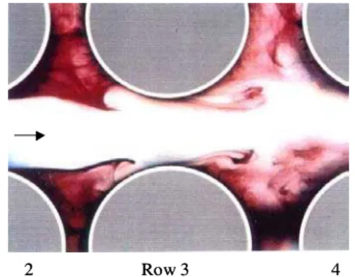
Figure 29. Flow patterns S1observed in a flow lane of a parallel triangle array. Xp = 1.44; Re = 580; water tests.
As in the staggered array case, the Strouhal number S2 is
associated with alternating vortex shedding behind the first two rows. This pattern, which is shown in Fig. 30, occurs only at relatively low Reynolds numbers. At higher Reynolds numbers, it is
replaced by the lowest vorticity component S1. As shown in Fig. 31,
this vorticity component, which is observed in arrays with Xp > 1.4,
is associated with large-scale alternating vortex shedding in the wakes of the inner tubes. At high Reynolds numbers, this vortex shedding component dominates in the whole array, i.e., it prevails also at the front rows.
Figure 30. Flow structure behind the front rows showing the vorticity shedding component S2. Parallel triangle array; Xp=2.08; Re = 1870.
Figure 31. Development of the flow structure associated with the vorticity component S1 in a parallel triangle array. Xp = 2.08; Re = 12300.
Strouhal Number of Vorticity Shedding in Parallel Triangle Arrays
The Strouhal numbers of vortex shedding in parallel triangle
arrays are given in Fig. 32. The Strouhal number in this chart is
based on the frequency of flow periodicity, fv, and the tube diameter,
d, as given by the Eq. (1). In this case, the gap velocity, Vg, is given
as a function of the upstream velocity Vu:
Vg = Vu [(2 Xp cos 30) / (2 Xp cos 30 - 1)] (6)
The Strouhal number data in Fig. 32 are seen to collapse mainly
around the three vorticity shedding components S1, S2 & S3.
Acoustic Strouhal Numbers in Parallel Triangle Arrays
predicted from the Strouhal numbers of the natural vorticity shedding, which are detected at non-resonant conditions. This feature is different from that of normal triangle arrays, but similar to the acoustic behavior of in-line arrays. This similarity seems to stem from the fact that both array patterns allow the flow to proceed freely along the flow lanes between the tube columns.
S1 S2
S3
Xp = P/d
S
tr
o
u
h
al
n
u
m
b
er
Parallel Triangle Arrays
S1 S2
S3
Xp = P/d
S
tr
o
u
h
al
n
u
m
b
er
Parallel Triangle Arrays
Figure 32. Strouhal number chart for vorticity shedding observed under non-resonant flow conditions in parallel triangle arrays.
In order to be able to predict the onset of acoustic resonance in parallel triangle arrays, an acoustic Strouhal number chart has been
developed and is given in Fig. 33. The acoustic Strouhal number, Sa,
is defined as:
Sa= fa d / Vg (7)
Where fa is the acoustic resonance frequency and Vg is the critical
gap velocity at the onset of acoustic resonance. As observed in Fig.
33, multiple acoustic Strouhal numbers exist in arrays with Xp<1.71.
Although some of these Strouhal numbers are associated with the resonance of all modes (from 1 to 3), some are related to only one mode. To avoid any misunderstanding, the acoustic modes excited by each Strouhal number are noted near each data point in Fig. 33. The curve displayed in this figure is the upper limit to the acoustic Strouhal numbers of the tested cases and should be treated as a design value to avoid acoustic resonances over the whole velocity range. In other words, the designer should ensure that the Strouhal number based on the maximum flow velocity and any acoustic frequency is higher than the design limit given by Fig. 33.
No resonance
Resonance
A
c
o
u
s
ti
c
S
tr
o
u
h
a
l
n
u
m
b
e
r
X
p= P/d
No resonance
Resonance
A
c
o
u
s
ti
c
S
tr
o
u
h
a
l
n
u
m
b
e
r
X
p= P/d
Figure 33. Acoustic Strouhal number chart for parallel triangle arrays. The acoustic modes excited are also provided near each data point.
The upper bound of the acoustic Strouhal numbers in Fig. 33 may appear similar to the envelope of the Strouhal numbers of the natural vortex shedding which are depicted in Fig. 32. However, this is true only for large spacing ratios, Xp > 2.3, which is to be expected, since alternating vortex shedding becomes dominant. For smaller spacing ratios, S3 can be up to 54% higher than the acoustic Strouhal number.
Summary
In general, except for in-line arrays, two or three distinct
frequency components of vortex shedding, fv1, fv2 and a third one,
are observed. The components fv2 and fv1 (fv2 > fv1) are found to be
associated with alternating vortex shedding from the tubes in the front and the rear rows, respectively. The third component is rather weak and appears at the front rows and at low Reynolds numbers only. The nature of all vortex shedding components and the relative importance of each one depend on the spacing ratio, the Reynolds number and the location within the array.
For staggered arrays, both components of vortex shedding, fv2 and fv1, are strong in the intermediate spacing case. However, the
lower component fv1 develops over the whole depth of the array at
high Reynolds numbers. Increasing the spacing ratio weakens the
high-frequency component fv2 at the front rows, until the
lower-frequency component fv1 dominates also at the front rows. The
opposite occurs when the spacing ratio is reduced, however, the
component fv2 remains confined to the front rows only.
In-line tube arrays are dominated by the symmetric instability of the jets issuing between the tube columns. This mode of vorticity shedding persists over the whole depth of intermediate spacing arrays. The flow activities in adjacent wakes or flow lanes are found to be well correlated and to satisfy well-defined phase relations. Due to these features, this vortex shedding mode is regarded as a ”global" mode of flow instability. As the tube spacing ratio is reduced, the jet instability and its spatial correlations are weakened. When the spacing ratio is increased, alternating wake shedding becomes the dominant mode of flow instability, especially if the upstream turbulence level is high.
Regarding acoustic resonances, it is shown that they are excited
by the natural vorticity shedding excitation in the cases of normal
triangle and rotated square arrays. In these cases, the Strouhal number charts of vorticity shedding, which are presented in this paper, can be used to design against tube vibration and acoustic resonance of the container.
For in-line and parallel triangle arrays, the occurrence of acoustic resonance is not related to the natural vortex shedding phenomenon which is observed in the absence of resonance. This conclusion is valid for arrays with small and intermediate spacing ratios, but it does not apply for arrays with relatively large spacing ratios. It is therefore necessary to use the acoustic Strouhal number chart to design against acoustic resonance and employ the vorticity shedding chart to avoid resonant vibration of the tubes. These design charts are also presented in this article.
References
Axisa, F., Antunes, J. and Villard, B., 1990, “Random Excitation of heat exchanger tubes by cross-flows”, Journal of Fluids and Structures, Vol. 4, pp. 321-341.
Bajaj, A. K. and Garg, V. K., 1977, “Linear stability of jet flows”, Journal of Applied Mechanics, Vol. 44, pp. 378-384.
Blevins, R. D. and Bressler, M. M., 1987a, “Acoustic resonance in heat exchanger tube bundles-Part I: physical nature of the problem”, Flow Induced Vibration 1987, PVP-Vol.122 (eds. M. K. Au-Yang & S. S. Chen), pp. 19-26. New York: ASME.