www.nat-hazards-earth-syst-sci.net/15/2299/2015/ doi:10.5194/nhess-15-2299-2015
© Author(s) 2015. CC Attribution 3.0 License.
The effect of uncertainty in earthquake fault parameters on the
maximum wave height from a tsunami propagation model
D. Burbidge1, C. Mueller2, and W. Power2
1Geoscience Australia, Canberra, Australia, now at GNS Science, Lower Hutt, New Zealand 2GNS Science, Lower Hutt, New Zealand
Correspondence to:D. Burbidge ([email protected])
Received: 26 March 2015 – Published in Nat. Hazards Earth Syst. Sci. Discuss.: 22 May 2015 Revised: 23 September 2015 – Accepted: 24 September 2015 – Published: 12 October 2015
Abstract.Over the last decade precomputed tsunami propa-gation model databases have been used extensively for both tsunami forecasting and hazard and risk assessment. How-ever, the effect of uncertainty in the earthquake source pa-rameters on the results of the simulated scenarios of tsunami propagation has not always been examined in great detail. Here we have undertaken a systematic study of the uncer-tainty in the maximum wave height of a tsunami (hmax) as a
function of the uncertainty in the rupture parameters of the earthquake that generates it (specifically the strike, dip, rake, depth and magnitude). We have shown that even for the sim-ple case of a tsunami propagating over flat bathymetry, the coefficient of variation (CoV) and skewness of the distribu-tion ofhmaxwas a complex function of the choice of rupture
parameter, distance and azimuth. The relationships between these parameters and CoV became even more complex as the bathymetry used became more realistic. This has major po-tential implications for both how warning centres operate in the future and how the uncertainty in parameters describing the source should be incorporated into future probabilistic tsunami hazard assessments.
1 Introduction
Since the 2004 Indian Ocean tsunami, there has been a major increase globally in tsunami propagation modelling for use in both tsunami warning and hazard and risk assessment. Prob-abilistic tsunami hazard assessments (PTHAs) have been cre-ated for the United States (Geist and Parsons, 2006; González et al., 2009), Australia (Burbidge et al., 2008, 2009), New Zealand (Power et al., 2007; Power, 2013), the
Mediter-ranean (Sørensen et al., 2012; Lorito et al., 2015), the north-west Indian Ocean (Heidarzadeh and Kijko, 2011), Indonesia (Horspool et al., 2014) and the even the entire globe (Løvholt et al., 2014). At the same time, hundreds to thousands of simulated scenarios of tsunami propagation have been cre-ated to inform real-time tsunami forecasting and alerts (e.g. Greenslade et al., 2007, 2013).
One aspect that has not been studied in great detail is the sensitivity, or uncertainty, in the maximum tsunami wave height due to uncertainty in the earthquake’s geometrical source parameters such as strike, dip and rake. Here we present a systematic study of this issue, starting with sim-ple source models in a flat ocean and then moving on to three examples which use a more realistic bathymetry.
Previous studies into what affects the tsunami wavefield have mostly focused on various physical parameters such as source effects (Geist, 1999), bathymetry (Geist, 2009), tides (Weisz and Winter, 2005), dispersion of wave propagation (Glimsdal et al., 2013), Coriolis force (Shuto, 1991), effects of friction (Myers and Baptista, 2001) and land cover rough-ness when propagating onshore (Kaiser et al., 2011). The ac-curacy of tsunami simulation not only depends on the con-sideration of these factors in the numerical implementation, but also on the variability and uncertainties associated with them.
distances. The particular type of numerical implementation, e.g. the choice of wave equation (linear and non-linear shal-low water wave equations, Boussinesq-type or full Navier– Stokes equations) and their corresponding capacity to incor-porate the factors mentioned above also has an influence on the accuracy of the simulation. Glimsdal et al. (2013) also found that dispersion is also a function of the dominant wave-length of the tsunami and the depth of the water at the source. The maximum amplitude of a tsunami in the near and far field has been investigated by several authors. Geist (2009) found that the maximum tsunami amplitude in the near field was mostly due to either the direct wave or edge waves along the continental shelf. By contrast, in the far field, the maximum amplitude was most often caused by a combination of source radiation pattern, scattering, reflec-tions and the nearshore response (edge waves, shelf modes and resonance). This work was continued in Geist (2012) who showed that far-field amplitude scaled with scalar seis-mic moment but with significant uncertainty in the correla-tion. Other studies, such as Davies et al. (2015), McCloskey et al. (2007, 2008), Løvholt et al. (2012) or Goda et al. (2014), have investigated the effect of non-uniform slip on the nearshore maximum tsunami height or on the maximum inundation height. However, these studies have generally fo-cused on one particular location and thus on a limited range of distances and azimuths. In Geist (2002), the effect of non-uniform slip on the far field was stated to be “less than 10 %” but the exact azimuth and distance at that point was not dis-cussed.
Having a better understanding of the uncertainty in the maximum tsunami wave height has the potential to be im-portant, not only for future tsunami hazard assessments but also tsunami forecasting and source inversions. In PTHAs it might be possible to treat the uncertainty in source parame-ters as an aleatory, rather than epistemic and include it in a probabilistic assessment, as discussed by Geist and Parsons (2006) or Thio et al. (2010). While in some cases this may be more computationally efficient, it may not be strictly correct according to the normal definition of those terms. Epistemic uncertainty, as defined by for example Marzocchi and Jor-dan (2014), is due to our lack of knowledge of the system, while aleatory uncertainty (or variability) is due to the in-trinsic randomness of the system. In theory, epistemic uncer-tainty can be reduced by more knowledge about the system, but aleatory uncertainty cannot. So uncertainty in, say, the dip is really an epistemic uncertainty, not an aleatory one, but in some cases it may be convenient to treat it as an aleatory uncertainty anyway.
Outside of hazard assessment, another potential use would be to know how close to a warning threshold a modelled tsunami wave height from an event must be in order for the difference to be “insignificant” given the current uncertainty in the source’s rupture parameters. This could then be used to inform the resulting warning given to the public. The un-certainty in source parameters could affect the reliability of
assumptions made, inverting for the source using tsunami mareogram data.
For the purposes of this paper, we have focused on try-ing to characterise the uncertainty in the maximum offshore tsunami wave height at a particular point (hmax). The reason
we have selected this particular model output is that this is the one most commonly used for both PTHAs and for tsunami alert threshold levels in warning systems.
The level of sensitivity in hmax to variations, or
uncer-tainties, in source properties can be measured in a variety of ways. Here we have quantitatively estimated this sensitiv-ity by calculating the coefficient of variation (CoV) ofhmax.
CoV was defined here to be equal toσmax/µmaxwhereσmax
was the corrected sample standard deviation andµmaxwas
the mean value ofhmaxat a particular location. Other metrics,
such asσ itself, could be used but CoV has the advantage of being both a dimensionless and reasonably common metric for estimating the dispersion of a distribution. We have esti-mated the CoV by runningN tsunami propagation models, each with a different value of a particular source parameter selected from a normal distribution with a standard deviation centred at the parameter’s mean. The normal distribution was chosen mainly for convenience as it is a simple, common ex-ample of an uncertainty distribution. The actual uncertainty distribution for some parameters could in fact be quite com-plex. For example, the uncertainty in the strike may vary with magnitude. However, in most cases, the correct distribution is not known and the normal distribution has the advantage of being simple. Given these assumptions,σmaxat a given point
is then
σmax(x, y)=
v u u t
1 N−1
N
X
i=1
hi
max(x, y)−µmax(x, y)2, (1)
wherehimax(x,y)was the maximum tsunami wave height at a particular location for theith model run.
earth-quake could not be entirely treated as a point source in the far field.
Okal and Synolakis (2008) also performed a few tests on the effect of shifting the epicentre and rake on maximum tsunami wave heights predicted from their numerical model. Again, this was only for a few examples and therefore can-not be used to calculate the CoV. However, they did con-clude from their study that the far-field pattern was robust to these variations. Okal and Synolakis (2004) also exam-ined the effect of varying a range of rupture parameters on the maximum run-up from nearshore events. However, they did not examine the CoV on the maximum run-up nor the effect on the maximum offshore wave height from more dis-tant events. In addition, Løvholt et al. (2012) examined the effect of changing the dip and depth on the CoV from a set of heterogeneous slip events using a plane wave tsunami model with idealised bathymetry. They found that the CoV of the maximum run-up from varying the slip decreased when the depth of the fault was increased but was unchanged when the dip was varied. However, they did not specifically look at the CoV from varying the bulk rupture parameters (eg strike, dip or depth) nor did they examine the effect of changing the dis-tance to the rupture or the azimuth. Xing et al. (2015) exam-ined the effect of strike, rake, dip and magnitude on the max-imum tsunami wave height at locations off the eastern coast of Australia for two tsunami sources, one on the New He-brides Trench and one on the Puysegur Trench. They found that hmax was changed when any of these parameters were
varied. However, these authors only studied five cases per parameter, and again the study was specific to a particular set of locations and sources. Finally, Goda et al. (2015) has recently published a study looking at the variation in inunda-tion footprints in the Tohoku region of Japan from different fault geometries (top edge depth, strike and dip) and slip dis-tributions. They found that the sensitivity to these parameters was highly dependent on tsunami source characteristics and site location and therefore complex and highly non-linear.
Here we have looked at how the CoV changes for a range of azimuths and distances for a given uncertainty in a partic-ular rupture parameter using one particpartic-ular tsunami propaga-tion model, EasyWave (Babeyko, 2012). The rupture param-eters chosen for this study were strike, dip, rake, magnitude and depth. The slip on all the models shown was uniform and the rupture dimensions were based on Abe (1975). We have done this in order to answer the following simple questions.
– Does the CoV vary with distance, azimuth or magnitude and how is it affected by bathymetry?
– Ishmaxnormally distributed? If not, is the shape of the
distribution also a function of distance, azimuth, magni-tude or bathymetry?
If the CoV does not vary significantly due to these factors and hmax was normally distributed, this could significantly
simplify both PTHAs and tsunami forecasting. The main
pur-pose of this paper is to see the extent to which we can assume that this is true for this particular set of examples.
2 Method
The method used here for assessing the uncertainty inhmax
was conceptually simple, if computationally intensive. It consisted of the following steps.
1. Choose a bathymetry.
2. Select a standard (or reference) set of rupture parame-ters.
3. Choose a random number from a normal distribution with a width given by the standard deviation in the pa-rameter to be studied (σstrike, σdip, σrake or σdepth
de-pending on the parameter).
4. Run the tsunami propagation model with this parameter and then save the maximum wave height at all points in the model’s domain.
5. Repeat steps 3 and 4 forN iterations, each with a dif-ferent, randomly generated, value of the parameter to be studied. Save the maximum wave heights at all points in the model for each iteration.
6. Use these models to calculateµmax across the model
domain.
7. Use Eq. (1) to calculateσmaxfor all points in the model
domain.
8. Calculate the ratio of σmax and µmax to calculate the
CoV at every point in the domain. 9. Map the resulting CoV values.
In addition to calculating the CoV, we have also binned theN models in order to examine the shape of the resulting distribution.
Finally, we have also mapped the sample skewness in or-der to provide a more quantitative measure of the shape of the distribution ofhmaxacross the model’s domain. The sample
skewness,S, was given by (Mantalos, 2010)
S= 1 N
N
P
i=1
himax−µmax 3
1 N
N
P
i=1
hi
max−µmax 2
3/2. (2)
is evenly distributed around the mean (as it would be for the normal or uniform distribution for example). Maps ofS al-lowed us to see whether the shape of distribution of hmax
changed with azimuth or distance.
For the studies shown here, we have setN=100. To test that this was adequate, we ran one set of runs with N=50
and found that this changed the maximum CoV in a test model by 11 %. However, when we ran one set of models withN=200, we found that this changed the maximum CoV
observed in the model by less than 1 %. ThereforeN=100
was chosen as a reasonable balance between accuracy in the maps and computational speed.
2.1 Bathymetry
For this study we used three increasingly complex bathymetry data sets. The first was a 80◦
×80◦bathymetry
model with a constant depth of 3678 m (the average depth of the ocean, Charette and Smith, 2010). The boundaries of the model go from −140 to 140◦ in longitude and from −40 to 40◦in latitude. The second bathymetric data set was
an 80◦ latitude by 42◦ longitude bathymetry model with a
constant depth of 3678m up until a step up in the elevation to 100 m a.m.s.l. (above mean sea level) near the eastern edge of the model domain. This model went from 140 to 181.25◦
in longitude but had the same range in latitude. The step at effectively acts as a reflecting wall. Both models were calcu-lated on a 4 arcmin grid. The first bathymetry can be viewed as a simplified version of the bathymetry near an oceanic sub-duction zone and the second for a (highly) simplified conti-nental subduction zone. Having uniform bathymetry removes bathymetry variations from the problem and allows us to un-derstand the patterns in CoV better. The stepped model could be made more like an actual continental margin by (for ex-ample) including a sloped ramp up to 100 m. However, the main aim of this bathymetry is just to demonstrate the effect of a basic process, in this case a simple reflection, rather than be a demonstration of the effect of a continental margin on CoV or skewness.
Some models were also run with both a 2 arcmin and a 8 arcmin grid and in both cases there was only a small change in the maximum CoV observed in the model (less than 5 %). However, there were some minor changes in the pattern. Therefore some of the details in the maps shown later could be influenced by the numerical resolution of the grid. This could be due to the different levels of numerical dispersion in the models with different grid resolutions or because some of the details of the initial deformation pattern and subsequent waves were missed for the coarser resolutions. However, the overall pattern appeared to be independent of the model res-olution.
The final bathymetry model used consisted of two sub-sections of ETOPO2 global elevation model (NOAA, 2006). Both were calculated on a 2 arcmin grid. ETOPO2 is one of the standard bathymetry models commonly used for tsunami
propagation calculations. These models illustrated the effect of realistic bathymetry on the CoV andSmaps.
2.2 Reference fault parameters
The uniform and stepped bathymetry tsunami runs used a uniform slip model with a set of “standard” values. The stan-dard values were
– dip=20◦;
– strike=0◦;
– rake=90◦;
– depth to the top edge of the rupture=10 km.
When a parameter was varied randomly the standard value listed above was the random distribution’s mean.
The standard value of the dip was chosen to be 20◦as this
is a typical value for the average dip of the seismogenic part of a subduction zone (e.g. the average dip of the interface in Slab 1.0 of Hayes et al. (2012) varies from 8 to 30◦depending
on the zone). Since we are mainly interested in tsunamigenic earthquakes the rake was set to be pure thrust. Since the rake was pure thrust, variations around that value add a strike–slip component to the motion and thus will generally reduce the amplitude of the tsunami. The depth of the top edge was kept quite shallow (10 km) as a typical “worst” case scenario. As a reviewer pointed out, when the depth is this shallow and the slip is uniform the initial sea surface displacement will have a distinct (and probably artificial) peak. The strike was chosen to propagate the tsunami along the equator and minimise any distortions simply due to the map projection. It also made the north and south parts of the domain symmetric which is a check that the sampling is adequate.
The sea floor deformation created by these sources was calculated on 10×10 km patches (i.e. sub-faults) using the
Okada equations as implemented in EasyWave, and then summed. Given that all the models considered in this paper had uniform slip, a single large source could also have been used. Patches were used instead since the original intention was to compare the CoVs andhmaxdistributions from
uni-form and non-uniuni-form slip models using the same sized set of sub-faults. This turned out to not be required to demon-strate complexity in the uncertainty patterns. One aspect of using sub-faults is that there may be small edge effects in the initial sea surface displacement when compared to that which would have been produced by a single, larger fault.
The fault’s centroid was positioned at 180◦W, 0◦N and
the maximum width was assumed to be 150 km. Above this magnitude it was assumed that the displacement continues to scale proportionately with the fault length; this is known as the L-model (Scholz, 1982; Hanks and Bakun, 2002). Al-though other, more recent, scaling relations could have been used, this particular set of scaling relations had the advantage of already being implemented in the computational frame-work (see Sect. 2.3) and the effect of different scaling rela-tions onhmaxand CoV was not intended to be the main focus
of this study.
For the models which were run using the ETOPO2 bathymetry, the epicentre and mean strike used were those of the 2011 Kermadec earthquake, 2007 Solomon Islands earth-quake or the 2006 Java earthearth-quake. The strike of these mod-els was set to be equal to that for one of the nodal planes for these events calculated by the USGS. Note that only the epicentre and strike were based on these events; the dip and rake were kept the same as the flat and stepped bathymetry examples in order to aid comparison. These three locations were chosen as they are good examples of subduction zones from different tectonic environments and thus bathymetries. The Kermadec zone is on a fairly typical oceanic subduction zone, the Solomon Islands zone is an example of a zone with complex bathymetry in the source region (i.e. multiple small islands) and Java is a typical example of a continental sub-duction zone.
2.3 Numerical models and scripts
The tsunami propagation model used here was EasyWave (Babeyko, 2012). The main reason this particular model was chosen was that it has been optimised for computa-tional speed and is open-source (http://trac.gfz-potsdam.de/ easywave). The time step for all the models shown here was the one calculated automatically by EasyWave. For the pur-pose of the uncertainty calculations, the Coriolis effect was not included.
A robust and efficient framework was required to manage the large amount of data and the simulated scenarios this method produced. A Python-based object oriented applica-tion programming interface (API) was developed that aug-ments and drives the EasyWave tsunami simulation program. The API allowed us to automate this parameter study using EasyWave as the tsunami simulation kernel. All the source models investigated in this study were created and managed with this API. The API also managed simulation on GNS Science’s cluster used for the computations, i.e. it farmed simulation scenarios out to cluster and collected data after simulation completion.
All the subsequent post-processing, including the map generation, was calculated by a set of post-processing GMT scripts (Wessel et al., 2013). The output grids from Easy-Wave and for the statistics were a mix of Golden Software© format files produced by EasyWave and NetCDF format files created by GMT.
140˚ 160˚ 180˚ −160˚ −140˚ −40˚
−20˚ 0˚ 20˚ 40˚
0 1 2 3 4 5 6
Mean Maximum Wave Height
m
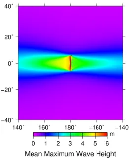
Figure 1.The mean of the maximum tsunami wave height (µmaxin
metres) for aMw=9.5 event with aσstrike=10◦. The bathymetry is uniform and completely flat. The earthquake’s rupture has a 20◦
dip to the right, its mean strike is north–south (i.e. 0◦), the depth
to the top edge is 10 km and it is centred at 180◦W, 0◦S. The slip
along the rupture plane is uniform and has a 90◦rake (i.e. it is a pure
thrust earthquake). The black box on the figure shows the surface projection of the mean rupture plane. The solid line on the left is the top edge of the plane and the dashed line on the right is the bottom edge.
3 Results
3.1 Uniform, flat bathymetry 3.1.1 Strike
Figure 1 shows the mean maximum wave height (hmax) over
100 uniform slip models withσstrikeof 10◦and a magnitude
ofMw=9.5. This level of uncertainty would be typical for a
well-constrained earthquake focal mechanism. The total ro-tational uncertainty (strike and dip) for a focal mechanism is typically between 5 and 20◦ (Kagan, 2003). The other
parameters are at their standard values (see Sect. 2.2). The bathymetry was flat with a uniform depth. As one might ex-pect, the tsunami propagated as two “beams”; one going to the east and one to the west of the earthquake rupture’s ini-tial location. The effect of averaging over 100 models with varying strike was that these beams become more “smeared” at their edges than they would be if only one model was sim-ulated.
Figure 2a–c shows maps of the CoV ofhmaxfrom three
sets of earthquakes with magnitudesMw=7.5, 8.5 and 9.5,
respectively. The sets of earthquakes varied in the strike by 10◦but were otherwise the same. As can be seen, the largest
foot-140˚ 160˚ 180˚ −160˚ −140˚ −40˚ −20˚ 0˚ 20˚ 40˚ (a)
0.0 0.1 0.2 0.3 0.4 CoV
140˚ 160˚ 180˚ −160˚ −140˚ −40˚ −20˚ 0˚ 20˚ 40˚ (b)
0.0 0.1 0.2 0.3 0.4 CoV
140˚ 160˚ 180˚ −160˚ −140˚ −40˚ −20˚ 0˚ 20˚ 40˚ (c)
0.0 0.1 0.2 0.3 0.4 CoV
140˚ 160˚ 180˚ −160˚ −140˚ −40˚ −20˚ 0˚ 20˚ 40˚ (d)
0.0 0.1 0.2 0.3 0.4 CoV
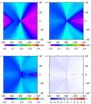
Figure 2.The effect ofσstrikeon the coefficient of variation (CoV)
ofhmax.(a)shows the CoV map from a set of 100 tsunami
gen-erated byMw=7.5 earthquakes which vary only in strike.(b)and
(c)show the effect on CoV when the magnitude of these events are increased toMw=8.5 andMw=9.5. For(a)–(c)σstrike=10◦. The bathymetry and other parameters are the same as in Fig. 1. Note that values above 0.4 are all shaded the same colour. 0.4 was chosen to be the maximum for these figures in order to be consistent with later figures.(d)shows the CoV map from a set ofMw=9.5 events with aσstrike=5◦.
wall (left) beam than for the hanging wall (right) beam for Mw=7.5 (Fig. 2a) but not for the higher magnitudes. The
variance was always at a minimum along strike (i.e. due north and south along the 180◦W line of longitude). The range
of CoV values went from 0.7 to 0.001 for Mw=9.5. For
Mw=7.5 it ranged from 0.3 to 0.001 but the bulk of the
re-gion was well below 0.2. For Mw=9.5 the most common
CoVs across the model domain were between 0.05 and 0.1 but many of the points were between 0.5 and 0.7 (histogram not shown, but this can be seen from the range of colour val-ues in Fig. 2c). Overall, the pattern was symmetric between the northern and southern halves of the model domain. How-ever, on close inspection some minor asymmetries were seen between the northern half of the model and the southern half, particularly due north and south of the earthquake’s epicen-tre. These are likely to be due to a combination of the finite number of samples and small numerical errors (e.g. round-off).
Just from this figure we can see that uncertainty in the strike makes the biggest difference (in terms of CoV) just off the main direction of the tsunami propagation. This means
0 5 10 15 20 25 30 35 40 45 50
Frequency
1 2 3 4
Maximum Wave Height (m) (a)
0 5 10 15 20 25 30 35 40 45 50
Frequency
1 2 3 4
Maximum Wave Height (m) (b)
0 5 10 15 20 25 30 35 40 45 50
Frequency
1 2 3 4
Maximum Wave Height (m) (c)
140˚ 160˚ 180˚ −160˚ −140˚ −40˚ −20˚ 0˚ 20˚ 40˚ (d)
A B C
−5 −4 −3 −2 −1 0 1 2 3 4 5 S
Figure 3.Example histograms for three locations surrounding a
Mw=9.5 event with aσstrike=10◦.(a)is at 160◦E, 0◦and is di-rectly in the mean path of the beam. This is an example of a location where the distribution has a strong negative skew.(b)is an example at the edge of the beam (160◦E, 5◦S). It is not skewed, but nor is
it normally or log-normally distributed.(c)is at 160◦E, 10◦S and
is thus just off the beam. This is an example of a location where the distribution of maximum wave heights has a strong positive skew. (d)shows the location of the histograms in(a)–(c)relative to the rupture. The background image shows the skewness (see Eq. 2) of the maximum tsunami wave height distribution across the domain.
an error in the strike in (for example) a tsunami forecast will make the largest difference to the amplitude in that location. Also, if one were to invert for the tsunami source, an obser-vation in these areas is likely to be much more helpful in constraining the strike rather than a point due north or south of the source.
Figure 2d shows the CoV map whenσstrikeis reduced to 5◦
for a magnitude ofMw=9.5. In this case, reducingσstrikedid
not change the pattern very much but reduced the amplitude and concentrated the larger CoV values into a smaller area. The maximum value of CoV reduced to 0.5 (down from 0.7). Also, the maximum effects of strike uncertainty occurred fur-ther from the source.
Figure 3a–c show the histogram of the maximum wave heights at locations A–C on Fig. 3d for aMw=9.5 event. As
140˚ 160˚ 180˚ −160˚ −140˚ −40˚ −20˚ 0˚ 20˚ 40˚ (a)
0.0 0.1 0.2 0.3 0.4 CoV
140˚ 160˚ 180˚ −160˚ −140˚ −40˚ −20˚ 0˚ 20˚ 40˚ (b)
0.0 0.1 0.2 0.3 0.4 CoV
140˚ 160˚ 180˚ −160˚ −140˚ −40˚ −20˚ 0˚ 20˚ 40˚ (c)
0.0 0.1 0.2 0.3 0.4 CoV
140˚ 160˚ 180˚ −160˚ −140˚ −40˚ −20˚ 0˚ 20˚ 40˚ (d)
−5 −4 −3 −2 −1 0 1 2 3 4 5 S
Figure 4. The effect ofσdipon the CoV and skewness ofhmax.
The magnitude of the earthquakes for each set were(a)Mw=7.5,
(b)Mw=8.5 or(c)Mw=9.5.σdip=5◦for all the sets shown here. The mean dip is 20◦. The strike is fixed to be due north–south. The
bathymetry and other parameters are otherwise the same as in Fig. 2 and are held constant for all 100 iterations.(d)The skewness of the distribution of the maximum tsunami wave heights for aMw=9.5 andσdip=5◦.
also shows the skewness values across the whole region more generally. The hmax distributions were generally positively
skewed, except for points in the beam close to the source where they were negatively skewed.
3.1.2 Dip
Figure 4a–c show the CoV maps when σdip is 5◦ for a
Mw=7.5, 8.5 and 9.5 events, respectively. Different plate
models typically differ by between 1 to 10◦in their estimates
of the average dip of an interface (e.g. see Table 1 in Hayes et al., 2012), so 5◦was chosen as a reasonable estimate of the
typical uncertainty in dip. The other parameters were held at their reference values.
Unlike the previous example, the maximum CoV was along strike (i.e. to the north and south of the epicentre) rather than to each side of the tsunami beam. So unlike the strike, an error in the dip has a bigger effect along strike than just off the main direction of propagation. For theMw=7.5
example it was also higher in the hanging wall direction (to the right of the figure) rather than the footwall direction. This difference became less strong (more concentrated into a smaller region) as the magnitude increased. The CoV ranged
140˚ 160˚ 180˚ −160˚ −140˚ −40˚ −20˚ 0˚ 20˚ 40˚ (a)
0.0 0.1 0.2 0.3 0.4 CoV
140˚ 160˚ 180˚ −160˚ −140˚ −40˚ −20˚ 0˚ 20˚ 40˚ (b)
0.0 0.1 0.2 0.3 0.4 CoV
140˚ 160˚ 180˚ −160˚ −140˚ −40˚ −20˚ 0˚ 20˚ 40˚ (c)
0.0 0.1 0.2 0.3 0.4 CoV
140˚ 160˚ 180˚ −160˚ −140˚ −40˚ −20˚ 0˚ 20˚ 40˚ (d)
−5 −4 −3 −2 −1 0 1 2 3 4 5 S
Figure 5.The effect ofσrake on the CoV and skewness ofhmax.
The magnitude of the earthquakes for each set were(a)Mw=7.5,
(b)Mw=8.5 or(c)Mw=9.5.σrake=20◦for all the sets shown here. The mean rake is 90◦. The bathymetry and other parameters
are otherwise the same as in the previous examples.(d)The skew-ness of the distribution of the maximum tsunami wave heights for a
Mw=9.5 andσrake=20◦.
from 0.4 to 0.01 for Mw=9.5 and from 0.2 to 0.002 for
Mw=7.5.
Figure 4d shows the skew pattern for theMw=9.5 case.
In this case the distributions were not as skewed as they were in the previous example. The skew was generally small and negative except immediately above the rupture where it was either strongly positive or negative.
3.1.3 Rake
Figure 5a–c show the CoV maps whenσrake is set equal to
20◦for aM
w=7.5, 8.5 and 9.5 event, respectively. Again,
this is typical uncertainty in a well-constrained focal mech-anism (e.g. see Shaw and Jackson, 2010). For theMw=7.5
case the regions of maximum CoV were on the hanging wall of the fault and on the footwall side forMw=8.5 and 9.5.
Unlike the previous two examples, the range of the CoV for theMw=9.5 andMw=7.5 events was essentially identical.
It ranged from 0.3 to 0.005 forMw=9.5 and from 0.3 to 0.04
forMw=7.5.
The skewness for theMw=9.5 set of events is shown in
140˚ 160˚ 180˚ −160˚ −140˚ −40˚ −20˚ 0˚ 20˚ 40˚ (a)
0.0 0.1 0.2 0.3 0.4 CoV
140˚ 160˚ 180˚ −160˚ −140˚ −40˚ −20˚ 0˚ 20˚ 40˚ (b)
0.0 0.1 0.2 0.3 0.4 CoV
140˚ 160˚ 180˚ −160˚ −140˚ −40˚ −20˚ 0˚ 20˚ 40˚ (c)
0.0 0.1 0.2 0.3 0.4 CoV
140˚ 160˚ 180˚ −160˚ −140˚ −40˚ −20˚ 0˚ 20˚ 40˚ (d)
−5 −4 −3 −2 −1 0 1 2 3 4 5 S
Figure 6.The effect ofσdepth (depth to the top edge of the
rup-ture) on the CoV and skewness of hmax. The magnitude of the
earthquakes for each set were (a) Mw=7.5, (b) Mw=8.5 or
(c)Mw=9.5.σdepth=2.5 km for all the figures shown here. The mean depth to the top edge was 10 km. The bathymetry and other parameters are otherwise the same as in the previous examples. (d)The skewness of the distribution of the maximum tsunami wave heights for aMw=9.5 and aσdepth=2.5 km.
3.2 Depth
Figure 6a–c show the CoV maps when the depth to the top edge of the fault was varied by aσdepthof 2.5 km for sets of
Mw=7.5, 8.5 and 9.5 events. Depths above 0 km were
re-jected to prevent “air quakes”. This uncertainty is fairly low for a typical earthquake, but was chosen to ensure that the distribution in depth is still approximately Gaussian after re-moving the “air quakes”.
These CoV maps had higher values on the hanging wall side than the footwall side for theMw=7.5 case (Fig. 6a).
The CoV was also generally higher forMw=7.5 than for the
other magnitudes. However, overall the CoV was much lower than for strike variations. The range of CoV went from 0.2 to 0.002 for theMw=9.5 set of events and from 0.2 to 0.03
forMw=7.5 set. However, the area covered with a high CoV
was much larger for the Mw=7.5 case than it was for the
Mw=9.5 case.
The skewness was negative on the footwall (left) side, pos-itive to the north and south of the rupture and mostly near zero on the hanging wall side for theMw=9.5 case (Fig. 6d).
140˚ 160˚ 180˚ −160˚ −140˚ −40˚ −20˚ 0˚ 20˚ 40˚ (a)
0.0 0.1 0.2 0.3 0.4 CoV
140˚ 160˚ 180˚ −160˚ −140˚ −40˚ −20˚ 0˚ 20˚ 40˚ (b)
0.0 0.1 0.2 0.3 0.4 CoV
140˚ 160˚ 180˚ −160˚ −140˚ −40˚ −20˚ 0˚ 20˚ 40˚ (c)
0.0 0.1 0.2 0.3 0.4 CoV
140˚ 160˚ 180˚ −160˚ −140˚ −40˚ −20˚ 0˚ 20˚ 40˚ (d)
−5 −4 −3 −2 −1 0 1 2 3 4 5 S
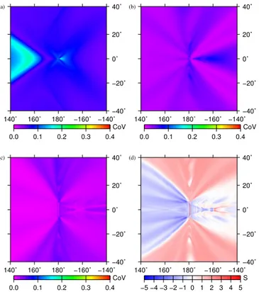
Figure 7.The effect of varying multiple fault parameters on the CoV and skewness. The magnitude of the earthquakes for each set were again (a) Mw=7.5, (b) Mw=8.5 or (c) Mw=9.5.
σstrike=10◦, σdip=5◦, σrake=20◦ and σdepth=2.5 km. The bathymetry and other parameters are otherwise the same as in the previous examples.(d)The skewness of the distribution of the max-imum tsunami wave heights for aMw=9.5 and theseσvalues.
Multiple parameters
The final example for the uniform bathymetry case we show here is one where all the parameters are allowed to vary around their reference values. In the example shown in Fig. 7, σstrike=10◦,σdip=5◦,σrake=20◦andσdepth=2.5 km. The
magnitudes varied betweenMw=7.5, 8.5 and 9.5. As one
might expect this pattern was a combination of all the pre-vious patterns; in this particular case it is dominated by the strike pattern, particularly for the higher magnitudes. The CoV ranged for Mw=9.5 from 0.6 to 0.1 and for
Mw=7.5 from 0.4 to 0.1. For Mw=9.5, skewness varied
from strongly positive to weakly negative depending on the azimuth (Fig. 7d).
3.3 Stepped bathymetry
Figure 8a shows what happens to a CoV map if a reflecting barrier is placed due east of the fault. In this particular exam-ple, we show the effect on the CoV for aMw=9.5 uniform
slip rupture withσstrike=10◦. As described in Sect. 2.1 the
bathymetry increased east of 182.5◦to 100 m a.s.l. (above sea
140˚ 160˚ 180˚ −40˚ −20˚ 0˚ 20˚ 40˚
(a)
0.0 0.1 0.2 0.3 0.4 CoV
140˚ 160˚ 180˚
−40˚ −20˚ 0˚ 20˚ 40˚
(b)
−5 −4 −3 −2 −1 0 1 2 3 4 5 S
Figure 8.The effect of having a step in the bathymetry on the CoV and skewness ofhmax.(a)shows the CoV from a set ofMw=9.5 events with aσstrike=10◦. The elevation has a step at 182.5◦where it suddenly increases to 100 m a.m.s.l. The other parameters are oth-erwise the same as in Fig. 2b. (b) The effect of the step on the skewness of the distribution of the maximum tsunami wave heights (cf. Fig. 3b).
regions just to each side of the beam had the highest CoV. The CoV also increased as one moved further away from the source. The range of the CoV for this example was from 0.5 to 0.001 just to the west of the epicentre.
Figure 8b shows the effect of this on the skewness field (cf. Fig. 3b). The areas to both sides of the beam were strongly positively skewed; those elsewhere were negatively skewed. The pattern also changed immediately above and to the west of the fault, where it was mostly positively skewed but with some areas which had a strong negative skewness.
3.4 Realistic bathymetry
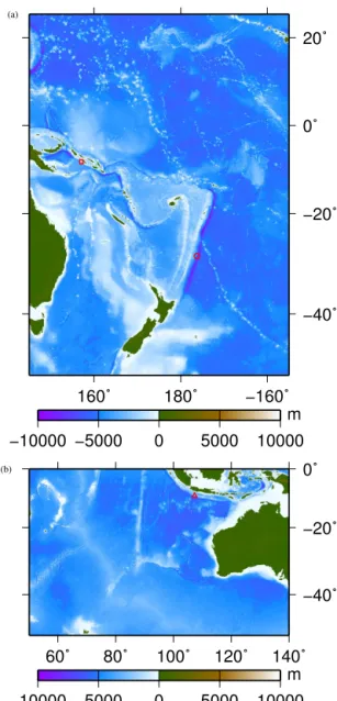
The previous examples all used flat or stepped bathymetric models. While this is very useful for determining basic pat-terns, in real cases, the bathymetry is highly non-uniform. Here we repeat some of the above experiments for hypothet-ical earthquakes on the Kermadec, Solomon Islands and Java subduction zones. The bathymetry used for these three ex-amples is shown in Fig. 9.
3.4.1 Kermadec event
Figure 10a–c shows the CoV maps for (a) σstrike of 10◦,
(b) σdip of 5◦ and (c) all the rupture parameters being
al-lowed to vary. The epicentre of the event was at 183.762◦E,
28.993◦S. The mean strike was 205◦. The other parameters
were the same as those list in Sect. 2.2. The magnitude is
160˚ 180˚ −160˚
−40˚ −20˚ 0˚ 20˚ (a)
−10000 −5000 0 5000 10000
m
60˚ 80˚ 100˚ 120˚ 140˚
−40˚ −20˚ 0˚ (b)
−10000 −5000 0 5000 10000
m
Figure 9.The bathymetry models used for the(a)Kermadec and Solomon Islands scenarios and(b)the Java scenario. The red sym-bols show the location of the epicentres for each scenario; a circle for the Kermadec scenario, a square for the Solomon Islands sce-nario and a triangle for the Java scesce-nario.
Mw=8.5 for all cases shown. For the last case, where
Figure 10. The CoV and skewness maps of hmax from a set
of earthquakes on the Kermadec Trench. Each set consisted of
Mw=8.5 earthquakes where either one parameter was allowed to vary (cases a or b) or all five were allowed to vary (case c). For (a)σstrike=10◦, for(b)σdip=5.0◦and for(c)σstrike=10◦,
σdip=5◦,σrake=20◦andσdepth=2.5 km.(d)The skewness map for case c.
with some shallow bathymetry between them and the source. The CoV in Fig. 10 ranges from 0.5 to 0.04.
Figure 10 shows the skewness values for the last case (where all parameters allowed to vary). Skewness was gener-ally non-zero and was neither consistently positive nor nega-tive but rather varied across the region.
3.4.2 Java event
Figure 11a–c show the CoV maps for an event off Java with the same set ofσ values used in the previous example. The epicentre of the event was at 107.33◦E, 9.32◦S. The mean
strike was 295◦. Again the broad pattern was similar to that
found from the uniform or stepped bathymetry models, but this ceased as soon as any complex bathymetry was reached. For example, the lines of maximum CoV split as the tsunami went around the southwest corner of Western Australia. The CoV range for Fig. 11c was 0.5 to 0.05.
60˚ 80˚ 100˚ 120˚ −40˚ −20˚ 0˚ (a)
0.0 0.1 0.2 0.3 0.4 CoV
60˚ 80˚ 100˚ 120˚ −40˚ −20˚ 0˚ (b)
0.0 0.1 0.2 0.3 0.4 CoV
60˚ 80˚ 100˚ 120˚ −40˚ −20˚ 0˚ (c)
0.0 0.1 0.2 0.3 0.4 CoV
60˚ 80˚ 100˚ 120˚ −40˚ −20˚ 0˚ (d)
−5 −4 −3 −2 −1 0 1 2 3 4 5 S
Figure 11.The CoV and skewness maps ofhmax from a set of
earthquakes on the Java subduction zone. Each set consisted of
Mw=8.5 earthquakes where either one parameter was allowed to vary (cases a or b) or all five were allowed to vary (case c). For(a)σstrike=10◦, for(b) σdip=5.0◦and for(c)σstrike=10◦,
σdip=5◦,σrake=20◦andσdepth=2.5 km.(d)The skewness map for case c.
Figure 11d shows the skewness pattern for this case. Again the pattern was only similar to the one found with flat bathymetry until the wave reached complex bathymetry. 3.4.3 Solomon Islands event
Finally we show an example of the CoV where the bathymetry is complex in the source region, in this case the Solomon Islands subduction zone (Fig. 12). The epicentre of the event was at 157.06◦E, 8.43◦S. The mean strike was
333◦. The basic patterns of flat bathymetry examples can now
barely be seen, if at all. The highly complex bathymetry in the source made predicting the CoV pattern at a given loca-tion difficult, if not impossible. The skewness map (Fig. 12d) is similarly complex. The highest CoV and skewness value were, in this case, due north of the earthquake’s epicentre. The CoV ranged from 0.8 to 0.04 (Fig. 12c). The maximum CoV was significantly higher in this case than for the other two examples, even though theσ values for the various pa-rameters were the same. However, the area of extremely high CoV values were very small.
4 Discussion
Figure 12.The CoV and skewness maps ofhmaxfrom a set of
earth-quakes on the Solomon Islands subduction zone. Each set consisted ofMw=8.5 earthquakes where either one parameter was allowed to vary (cases a or b) or all five were allowed to vary (case c). For (a)σstrike=10◦, for(b)σdip=5.0◦and for(c)σstrike=10◦,
σdip=5◦,σrake=20◦andσdepth=2.5 km.(d)The skewness map for case c.
For points with the beam (i.e. in the main direction of tsunami propagation) any change in strike, positive or negative, will always act to reduce the hmax. For points outside the beam
any change would reduce hmax. Thus the distribution was
negatively skewed in the beam and positively skewed out-side of it (Fig. 3). The magnitude of this effect will be at its greatest for points just outside the beam since they can go from being entirely inside the beam to entirely outside of it with just a small change in strike. Thus the CoV was at a maximum there (Fig. 2).
However, the patterns in the other cases are not as intuitive. Having the maximum CoV along strike when the dip was varied is due to the way the dip changes the initial crustal de-formation pattern by bringing the line of displacement closer to the trench. In a similar way, the other changes in CoV are due to the way changes in other parameters affect the initial deformation pattern.
The fact that the patterns and values change with magni-tude suggests strongly that these effects are also linked to
the changing dimensions and aspect ratio of the source re-gion. At lower magnitudes (Mw=7.5 in our examples) the
source appears to be “point-like” except in the near field. At intermediate magnitudes (Mw=8.5 in our examples) the
source dimensions mean that the source is more “area-like”. At large magnitudes (Mw=9.5 in our example) the aspect
ra-tio changes such that the length becomes much greater than the width, and the source becomes “line-like” in the far field. The reduced sensitivity to uncertainty in depth between Mw=7.5 andMw=8.5 can be understood in this context. At
Mw=7.5 the rupture width was small and therefore occupies
a small range of depths, so uncertainty in the depth of the top edge made a significant change to the overall deforma-tion pattern and subsequent tsunami. However atMw=8.5
the larger rupture surface already occupies a wide range of depths, so uncertainty in the depth of the top edge made pro-portionately less difference overall.
A result of this complexity is that it is very difficult to make general statements about the level of uncertainty in hmax given an uncertainty in any of the source parameters.
For some particular locations or azimuths a small uncertainty in strike made very little difference to the result (i.e. less than 10 %); in other locations it changedhmaxby 20 % or even by
more than 50 % (Fig. 2). It all depended on the azimuth, and for the latter examples, the bathymetry between the source and the location. This is broadly consistent with Gica et al. (2007) where the same 10◦change in strike could change the
wave height measured at Hawaii by between 12 and 84 %; depending on the location of the earthquake relative to the island. When the bathymetry in the source location was com-plex, such as in the Solomon Islands case (Fig. 12), the CoV and skewness maps became impossible to distinguish from noise and only general statements about the maximum upper bound on the CoV orScan really be made.
Initially, the authors assumed that it might be possible to treat the uncertainty in the source parameters as an aleatory, rather than epistemic uncertainty in PTHAs as discussed in the Sect. 1. However, our study shows that includingσ un-certainties in PTHAs as aleatory uncertainty can only ever be very approximate. It will always be difficult to be sure whether the values used are not over- or underestimating the hazard at a particular location given the highly, and incon-sistently, skewed distributions ofhmax. Since the skew can
change from positive to negative over very short length scales these issues cannot be simply solved by using a different type of σ (e.g. a log-normal σ). The ideal solution clearly has to be to run a large number of models to try to ensure that the hazard from the events in any tails of these skewed dis-tributions are included in the assessment. However, this can become very computationally challenging for larger assess-ments.
currently include any assessment of the spatial distribution of the CoV for each scenario, although the CoV between differ-ent scenarios has been calculated (Greenslade et al., 2013). Given the large number of possible events, calculating the CoV for each event would be an extremely large computa-tional task. It was also noticeable that the CoV distribution for events involving realistic bathymetry tends to become very scattered in shallow coastal areas outside of the near field, possibly the result of complex interference patterns in-volving multiple waves. This is similar to the scattering in hmax from shallow bathymetric features observed by
Mof-jeld et al. (2004). Another explanation might be that the res-olution of the grids used in our study was not high enough in the coastal regime to properly assess the CoV. In either case, many forecast methodologies rely on warning zones, which are sections of coast in which a warning threshold is crossed once a particular proportion of maximum wave heights (e.g. the 95th percentile) exceeds a specified level (e.g. Uslu and Greenslade, 2013). An area for further study is to see to what extent thresholds defined in these aggre-gate terms are sensitive to uncertainties in source parameters. If this does effect the reliability of thresholds, it therefore seems advisable to move away from precalculated tsunami databases and use fast tsunami simulation programs instead that allow for the calculation of both the CoV andµmaxas the
tsunami event unfolds (i.e. ensemble forecasting). The CoV and the shape of the distribution ofhmaxfrom this ensemble
of models can then inform about the reliability of the tsunami forecast (and thus the warning) for any given point of inter-est. It also suggests that warnings should try to move towards taking uncertainties in the source into account more directly in the warning, for example using Bayesian networks (Blaser et al., 2011, 2012).
In addition to the potential issues just discussed, our re-sults also indicate that the inversion of the tsunami source based on DART®buoy information will be affected by the relative positions of the source and the DART®buoys. If a DART® buoy happens to be located in an area that has a low CoV for a particular fault parameter, we would expect the resulting inversion for that parameter to be poorly con-strained. In other words, the inverted source is non-unique. For example, if the inversion only has DART®buoys close to aMw=9.5 earthquake, the maximum wave height at those
DART®buoys will not be significantly affected by an error in strike unless one of them happens to be close to the edge of the rupture (see Fig. 2c–d). Thus the strike may not be well-constrained. However, the same error in strike could make a large difference in the observed maximum wave height fur-ther from the source (i.e. in the red areas in Fig. 2c–d). This is consistent with the observation of Wang (2008) that gauges off the centre line of the tsunami propagation are more use-ful for constraining the source than those in tsunami beam itself. Ultimately, this sort of effect will create more uncer-tainty in the predicted wave fields. Reducing the unceruncer-tainty ideally requires techniques which can measure the tsunami
wave height over broad areas (e.g. using remote sensing) or include additional types of data (e.g. seismic or geodetic). Also many inversion algorithms assume a Gaussian or log-normal distribution of misfits; as can be seen from the maps of skewness, this is not always the case. The effect of this on tsunami inversion assumptions is also be another potential area of future research.
5 Conclusions
The main conclusion of this study is that “the uncertainty in the maximum wave height of a tsunami is a complex function of our uncertainty in the source parameters and bathymetry”. Even for the case of a completely flat bathymetry, complex patterns of CoV and skewness were seen. These patterns be-came even more complex when realistic bathymetries were used. While the specifics of these CoV maps may be influ-enced by the particular choice of numerical and bathymetry models used here, the overall patterns are probably not. For example, the high CoV lobes to each side of the beam when the strike was varied appear to be a function of the beam-like nature of tsunami propagation. Thus any model or bathymetry is likely to have a broadly similar CoV map even if the details may be different.
Given the complexity of CoV (and thus σ), simplified methods of taking earthquake uncertainty into account in PTHAs have the potential to be quite inaccurate. Depend-ing on the wayσ or CoV is chosen, they will overestimate the hazard in some locations and underestimate it in others. Also,σ does not follow a simple-normal or log-normal dis-tribution as shown by the fact that the skewness also changes with distance and azimuth. This suggest that the best way to incorporate uncertainty in earthquake parameters in fu-ture PTHAs is still to model all reasonably possible earth-quake ruptures. Similarly, these results give further impetus towards using real-time ensemble tsunami propagation mod-els for warnings, rather than relying on limited catalogues of possible future tsunamis. The already substantial compu-tational task of both activities will thus likely need to grow even further in future in order to take uncertainties such as these into account.
Author contributions. D. Burbidge ran the models, wrote the scripts for analysing the results, prepared the figures, wrote the bulk of the text and the response to reviewers. C. Mueller wrote the Python API which managed the simulations. Both C. Mueller and W. Power contributed text to the final version of the manuscript, mostly to the Introduction, Method and Discussion sections.
the three anonymous referees and X. Wang, N. Horspool and J. Sexton for reviewing this document. The paper is published with the permission of the CEO of Geoscience Australia.
Edited by: I. Didenkulova
Reviewed by: three anonymous referees
References
Abe, K.: Reliable estimation of the seismic moment of large earth-quakes, J. Phys. Earth, 23, 381–390, 1975.
Babeyko, A.: EasyWave: fast tsunami simulation tool for early warning, http://trac.gfzpotsdam.de/easywave (last access: 13 May 2015), 2012.
Blaser, L., Ohrnberger, L. M., Riggelsen, C., Babeyko, A., and Scherbaum, F.: Bayesian networks for tsunami early warning, Geophys. J. Int., 185, 1431–1443, 2011.
Blaser, L., Ohrnberger, M., Krüger, F., and Scherbaum, F.: Proba-bilistic tsunami threat assessment of 10 recent earthquakes off-shore Sumatra, Geophys. J. Int., 188, 1273–1284, 2012. Burbidge, D., Mleczko, R., Thomas, C., Cummins, P., Nielsen, O.,
and Dhu, T.: A Probabilistic Tsunami Hazard Assessment for Australia, Geoscience Australia Professional Opinion 2008/04, Canberra, Australia, 2008.
Burbidge, D., Cummins, P. R., Mleczko, R., and Thio, H. K.: A probabilistic tsunami hazard assessment for Western Australia, Pure Appl. Geophys., 165, 2059–2088, 2009.
Charette, M. A. and Smith, W. H. F.: The Volume of Earth’s Ocean, Oceanography, 23, 112–114, 2010.
Dao, M. H. and Tkalich, P.: Tsunami propagation modelling – a sensitivity study, Nat. Hazards Earth Syst. Sci., 7, 741–754, doi:10.5194/nhess-7-741-2007, 2007.
Davies, G., Horspool, N., and Miller, V.: Tsunami inundation from real heterogeneous earthquake slip distributions: Evaluations of synthetic source models, J. Geophys. Res.-Solid Ea., 120, doi:10.1002/2015JB012272, in press, 2015.
Geist, E. L.: Local tsunamis and earthquake source parameters, Adv. Geophys., 39, 117–209, 1999.
Geist, E. L.: Complex earthquake rupture and local tsunamis, J. Geophys. Res.-Solid Ea., 107, 2-1–2-15, doi:10.1029/2000JB000139, 2002.
Geist, E. L.: Phenomenology of tsunamis: Statistical proper-ties from generation to runup, Adv. Geophys., 51, 107–169, doi:10.1016/S0065-2687(09)05108-5, 2009.
Geist, E. L.: Phenomenology of tsunamis II: Scaling, Event Statis-tics, and Inter-Event Trigeering, Adv. Geophys., 53, 35–92, doi:10.1016/B978-0-12-380938-4.00002-1, 2012.
Geist, E. L. and Parsons, T.: Probabilistic Analysis of Tsunami Haz-ards, Nat. HazHaz-ards, 37, 277–314, doi:10.1007/s11069-005-4646-z, 2006.
Gica, E., Teng, M. H., Liu, P. L.-F., Titov, V., and Zhou, H.: Sensi-tivity Analysis of Source Parameters for Earthquake-Generated Distant Tsunamis, J. Waterway Port Coast. Ocean Eng., 133, 429–441, 2007.
Glimsdal, S., Pedersen, G. K., Harbitz, C. B., and Løvholt, F.: Dispersion of tsunamis: does it really matter?, Nat. Hazards Earth Syst. Sci., 13, 1507–1526, doi:10.5194/nhess-13-1507-2013, 2013.
Goda, K., Mai, P. M., Yasuda, T., and Mori, N.: Sensitivity of tsunami wave profiles and inundation simulations to earthquake slip and fault geometry for the 2011 Tohoku earthquake, Earth Planets Space, 66, 1–20, doi:10.1186/1880-5981-66-105, 2014. Goda, K., Yasuda, T., Mori, N., and Mai, P. M.: Variability of
tsunami inundation footprints considering stochastic scenarios based on a single rupture model: Application to the 2011 To-hoku earthquake, J. Geophys. Res.-Oceans, 120, 4552–4575, doi:10.1002/2014JC010626, 2015.
González, F., Geist, E., Jaffe, B., Kânoglu, U., Mofjeld, H., Syn-olakis, C., Titov, V., Arcas, D., Bellomo, D., Carlton, D., Horn-ing, T., Johnson, J., Newman, J., Parsons, T., Peters, R., Peterson, C., Priest, G., Venturato, A., Weber, J., Wong, F., and Yalciner, A.: Probabilistic tsunami hazard assessment at Seaside, Oregon for near- and far-field seismic sources, J. Geophys. Res., 114, C11023, doi:10.1029/2008JC005132, 2009.
Greenslade, D. J. M., Simanjuntak, M. A., Burbidge, D., and Chit-tleborough, J.: A first-generation real-time tsunami forecasting system for the Australian region, BMRC Research Report 126, Bureau of Meteorology, Melbourne, Australia, 2007.
Greenslade, D. J. M., Annunziato, A., Babeyko, A., Burbidge, D., Ellguth, E., Horspool, N., Srinivasa Kumar, T., Kumar, C. P., Moore, C., Rakowsky, N., Riedlinger, T., Ruangrassamee, A., Srivihok, P., and Titov, V. V.: An Assessment of the Diversity in Scenario-based Tsunami Forecasts for the Indian Ocean, Cont. Shelf Res., 79, 36–45, 2013.
Hanks, T. C. and Bakun, W. H.: A bilinear source-scaling model for M-log A observations of continental earthquakes, Bull. Seismol. Soc. Am., 95, 1841–1846, 2002.
Hayes, G. P., Wald, D. J., and Johnson, R. L.: Slab1.0: A three-dimensional model of global subduction zone geometries, J. Geophys. Res., 117, B01302, doi:10.1029/2011JB008524, 2012. Heidarzadeh, M. and Kijko, A.: A probabilistic tsunami hazard as-sessment for the Makran subduction zone at the northwestern Indian Ocean, Nat. Hazards, 56, 577–593, doi:10.1007/s11069-010-9574-x, 2011.
Horspool, N., Pranantyo, I., Griffin, J., Latief, H., Natawidjaja, D. H., Kongko, W., Cipta, A., Bustaman, B., Anugrah, S. D., and Thio, H. K.: A probabilistic tsunami hazard assessment for Indonesia, Nat. Hazards Earth Syst. Sci., 14, 3105–3122, doi:10.5194/nhess-14-3105-2014, 2014.
Kagan, Y. Y.: Accuracy of modern global earthquake catalogs, Phys. Earth Planet. Int., 135, 173–209, 2003.
Kaiser, G., Scheele, L., Kortenhaus, A., Lovholt, F., Romer, H., and Lesdchka, S.: The influence of land cover roughness on the re-sults of high resolution tsunami inundation modeling, Nat. Haz-ards Earth Syst. Sci., 1, 2521–2540, doi:10.5194/nhess-11-2521-2011, 2011.
Lorito, S., Selva, J., Romano, F., Tiberti, M. M., and Piatanesi, A.: Probabilistic hazard for seismically induced tsunamis: accuracy and feasibility of inundation maps, Geophys. J. Int., 200, 574– 588, doi:10.1093/gji/ggu408, 2015.
Løvholt, F., Pedersen, G., Bazin, S., Kuhn, D., Bredesen, R. E., and Harbitz, C.: Stochastic analysis of tsunami runup due to hetero-geneous coseismic slip and dispersion, J. Geophys. Res., 117, C03047, doi:10.1029/2011JC007616, 2012.
United Nations Office for Disaster Risk Reduction, Geneva, Switzerland, 2014.
Mantalos, P.: Three Different Measures of Sample Skewness and Kurtosis and their Effects on the Jarque-Bera Test for Normal-ity, Jönköping International Business School Working Papers No. 2010-9, Jönköping University, Jönköping, Sweden, 2010. Marzocchi, W. and Jordan, T. H.: Testing for
ontologi-cal errors in probabilistic forecasting models of natu-ral systems, P. Natl. Acad. Sci. USA, 111, 11973–11978, doi:10.1073/pnas.1410183111, 2014.
McCloskey, J., Antonioli, A., Piatanesi, A., Sieh, K., Steacy, S., Nal-bant, S. S., Cocco, M., Giunchi, C., Huang, J. D., and Dunlop, P.: Near-field propagation of tsunamis from megathrust earthquakes, Geophys. Res. Lett., 34, L14316, doi:10.1029/2007GL030494, 2007.
McCloskey, J., Antonioli, A., Piatanesi, A., Sieh, K., Steacy, S., Nalbant, S., Cocco, M., Giunchi, C., Huang, J., and Dunlop, P.: Tsunami Threat in the Indian Ocean from a Future Megathrust Earthquake West of Sumatra, Earth Planet. Sc. Lett., 265, 61–81, 2008.
Mofjeld, H. O., Symons, C. M., Lonsdale, P., Gonzalex, F. I., and Titov, V. V.: Tsunami scattering and earthquake faults in the deep Pacific Ocean, Oceanography, 17, 38–46, 2004.
Myers, E. P. and Baptista, A. M.: Analysis of Factors Influencing Simulations of the 1993 Hokkaido Nansei-Oki and 1964 Alaska Tsunamis, Nat. Hazards, 23, 1–28, 2001.
NOAA: 2-minute Gridded Global Relief Data (ETOPO2v2), US Department of Commerce, National Oceanic and At-mospheric Administration, National Geophysical Data Cen-ter, http://www.ngdc.noaa.gov/mgg/fliers/06mgg01.html (last access: 8 October 2009), 2006.
Okal, E. A. and Synolakis, C. E.: Source discriminants for near-field tsunamis, Geophys. J. Int., 158, 899–912, 2004.
Okal, E. A. and Synolakis, C. E.: Far-field tsunami hazard from mega-thrust earthquakes in the Indian Ocean, Geophys. J. Int., 172, 995–1015, 2008.
Power, W.: Review of Tsunami Hazard in New Zealand (2013 Up-date), GNS Science Consultancy Report 2013/131, GNS Sci-ence, Lower Hutt, New Zealand, p. 222, 2013.
Power, W., Downes, G., and Stirling, M.: Estimation of Tsunami Hazard in New Zealand due to South American Earthquakes, Pure Appl. Geophys., 164, 547–564, doi:10.1007/s00024-006-0166-3, 2007.
Scholz, C. H.: Scaling laws for large earthquakes: consequences for physical models, Bull. Seismol. Soc. Am., 72, 1–14, 1982. Shaw, B. and Jackson, J.: Earthquake mechanisms and active
tec-tonics of the Hellenic subduction zone, Geophys. J. Int., 181, 966–984, 2010.
Shuto, N.: Numerical simulation of tsunamis? Its present and near future, Nat. Hazards, 4, 171–191, doi:10.1007/BF00162786, 1991.
Sørensen, M. B., Spada, M., Babeyko, A., Wiemer, S., and Grün-thal, G.: Probabilistic tsunami hazard in the Mediterranean Sea, J. Geophys. Res., 117, B01305, doi:10.1029/2010JB008169, 2012.
Thio, H. K., Somervile, P., and Polet, J.: Probabilistic Tsunami Hazard in California, Pacific Earthquake Engineering Research Center Report 2010/108, Pacific Earthquake Engineering Center, University of California, Berkeley, California, USA, 2010. Titov, V. V., Mofjeld, H. O., Gonzalez, F. I., and Newman, J. C.:
Off-shore forecasting of Alaska-Aleutian Subduction Zone tsunamis in Hawaii, NOAA Technical Memorandum ERL PMEL-114, NOAA, Seattle, 1999.
Uslu, B. and Greenslade, D. J. M.: Validation of Tsunami Warn-ing Thresholds UsWarn-ing Inundation ModellWarn-ing, CACWR Technical Report No. 062, The Centre for Australian Weather and Climate Research, Melbourne, Australia, 2013.
Wang, X.: Numerical modelling of surface and internal waves over shallow and intermediate water, PhD thesis, Cornell University, Ithaca, New York, 2008.
Weisz, R. and Winter, C.: Tsunami, tides and run-up: a numerical study, in: Proceedings of the International Tsunami Symposium, 27–29 June 2005, edited by: Papadopoulos, G. and Satake, K., Chania, Greece, p. 322, 2005.
Wessel, P., Smith, W. H. F., Scharroo, R., Luis, J., and Wobbe, F.: Generic Mapping Tools: Improved Version Released, EOS Trans. AGU, 94, 409–410, doi:10.1002/2013EO450001, 2013. Xing, H. L., Ding, R. W., and Yuen, D. A.: Tsunami Hazards along