* Corresponding author:
E-mail: [email protected]
Received: March 13, 2018
Approved: July 10, 2018
How to cite: Silva MLN, Libardi PL, Gimenes FHS. Soil water retention curve as affected by sample height. Rev Bras Cienc Solo. 2018;42:e0180058.
https://doi.org/10.1590/18069657rbcs20180058
Copyright: This is an open-access article distributed under the terms of the Creative Commons Attribution License, which permits unrestricted use, distribution, and reproduction in any medium, provided that the original author and source are credited.
Division - Soil Processes and Properties | Commission – Soil Physics
Soil Water Retention Curve as
Affected by Sample Height
Maria Laiane do Nascimento Silva(1)*, Paulo Leonel Libardi(2) and Fernando Henrique Setti Gimenes(1)
(1)
Universidade de São Paulo, Escola Superior de Agricultura “Luiz de Queiroz”, Departamento de Ciência do Solo, Programa de Pós-Graduação em Solos e Nutrição de Plantas, Piracicaba, São Paulo, Brasil.
(2)
Universidade de São Paulo, Escola Superior de Agricultura “Luiz de Queiroz”, Departamento de Engenharia de Biossistemas, Piracicaba, São Paulo, Brasil.
ABSTRACT: The soil water retention curve is one of the main instruments to assess the soil physical quality and to improve soil management. Traditionally, the equipment most used in the laboratory to determine the retention curve has been Haines funnels and Richards chambers. An important factor to which little attention has been given in the use of these equipaments is the height of the undisturbed soil sample. This work
proposes to evaluate the influence of different heights of undisturbed samples for the
determination of the retention curve. For this, undisturbed soil samples were collected
in aluminum cylinders of three different heights (S1 = 75 mm; S2 =50mm; S3 =25 mm)
and with the same internal diameter (70 mm) from the diagnostic horizons of a Typic
Hapludox and a Kandiudalfic Eutrudox (Latossolo Vermelho amarelo distrófico típico and
Nitossolo Vermelho eutrófico latossólico, respectively) in experimental areas of “Escola
Superior de Agricultura Luiz de Queiroz” (ESALQ/USP), Piracicaba (SP), Brazil. The soil physical characterization was done based on granulometric analysis, bulk density, particle density, porosity, and organic carbon. The retention curves were determined for each sample size using Haines funnels for the tensions of 0.5, 1, 4, 6, and 10 kPa and Richards
chambers for 33, 100, and 500 kPa. Data of the curves were estimated, fitted to a model and then the distribution of the soil pore radius was evaluated, differentiating the soil water retention curve. The Typic Hapludox showed a not so remarkable difference between
the retention curve with the S3 samples and the retention curve with the S1 samples, in the range 0-1 kPa of tensions, and also between the retention curve with S1 samples and both retention curves with the S2 and S3 samples, in the range 100-500 kPa of tension.
This led to a slight difference in the pore distribution curves for the sample heights of this soil. The Kandiudalfic Eutrudox, however, presented not only a remarkable difference of
the smaller sample retention curve (S3) in relation to the larger ones (S1 and S2) in the
range 0-10 kPa of tension, but also a notable difference in the pore distribution curves,
with a reduction of mesopores and increase of micropores with the increase of sample height. Finally, from the results obtained and with the methodology used to determine the soil retention curve, it is not recommended to use undisturbed samples with a height greater than 25 mm.
INTRODUCTION
The quantification of soil water flow is essential for several areas of agriculture, soil
science, and hydrology, such as irrigation and fertilizer management, remediation of
polluted areas, and many others. Specifically, the numerical solution for the Richards
equation requires, as input parameters, a knowledge of the soil water retention curve and soil hydraulic conductivity as a function of soil water content (Solone et al., 2012).
The retention curve has also become one of the main instruments in soil physics to understand how water moves and is retained in the soil (Ghanbarian et al., 2015). From this curve, important information such as the distribution of soil pore size and modeling of the porous medium for the prediction of hydraulic conductivity of unsaturated soil can be obtained (Burdine, 1953; Mualem, 1976; van Genuchten, 1980; Hunt et al.,
2013; Ghanbarian et al., 2015). Besides, the retention curve can be affected by specific
characteristics of each soil, such as the mineralogy of the clay fraction, organic matter, shape, and arrangement of soil particles, or the composition and concentration of solutes in soil solution, among others (Grohmann and Medina, 1962; Beutler et al., 2002).
When using instruments with a porous plate, such as Richards chambers and Haines
funnels, the retention curve can also be affected by hysteresis, temperature, hydraulic
conductance of the porous material, sample saturation contact between the sample, and porous plate, and the correct detection of the point of equilibrium of the water in the instrument at each selected tension (Klute, 1986; Moraes et al., 1993; Munoz-Carpena
et al., 2002; Abbasi et al., 2012; Solone et al., 2012). Remarkable differences between
the matric potential measured by instruments with a porous plate at high pressure and instruments using the dew point measurement was reported by Bittelli and Flury (2009). They found that the water coming out of the sample at the tension of 1,500 kPa was two times more than that determined with the dew point meter. This might be because of the
difficulty the water has in attaining equilibrium in such high tensions, in which the soil
hydraulic conductivity is very low, and the time the samples remained in the equipment may not have been enough to provide equilibrium conditions (Hunt and Skinner, 2005).
Richards chambers and Haines funnels are some of the most commonly used instruments for determining the soil water retention curve in the laboratory and, so far, little attention
has been given to the dimensions of the sample, specifically its height, when using these instruments. The influence of the sample size on the soil water retention curve by means of percolation theory was studied, and it was verified that smaller samples provided
greater accessibility between the pores of the interior and the pores of the surface of the sample (Larson and Morrrow, 1981; Zhou and Stenby, 1993). The diameter and height of samples were used as input in pedotransfer functions to obtain the soil water retention curve and the hydraulic conductivity of the saturated soil (Ghanbarian et al., 2015). The results showed that the inclusion of the dimensions of the sample as a parameter in the pedotransfer functions could improve the precision of the prediction of these soil properties.
According to the literature, the height of undisturbed soil samples used to determine the soil water retention curve varies from 0.03 to 0.075 m (Moraes et al., 1993; Claessen, 1997; Beutler et al., 2002; Machado et al., 2008; Brito et al., 2011). It is reported by Reichardt and Timm (2004) that the height of the samples for this type of analysis can vary from 0.03-0.10 m. By using the Haines funnel to determine the matric potential,
what is done is to impose a pressure difference across its porous plate by means of
suction beneath the plate (in the base of the sample), which may be a hanging water
column or a controlled vacuum. In the Richards chamber, a pressure difference is also
plate is used to maintain atmospheric pressure at the sample base and to support an air pressure greater than the atmospheric pressure acting on the sample through its
top. Therefore, the height of the sample over this point can influence the value of the
soil water content for a given matric potential. Thus, this work was developed with the
objective of assessing different heights of undisturbed sample to determine the soil water
retention curve by the traditional method using porous plate funnels (Haines funnels) and plate porous air pressure chambers (Richards chambers).
MATERIALS AND METHODS
Disturbed and undisturbed samples were collected from the diagnostic horizon of two soils located in experimental areas of the “Escola Superior de Agricultura Luiz Queiroz”
(Esalq/USP), Piracicaba, São Paulo. The soils were classified by Cooper et al. (2002) according to the Soil Taxonomy (Soil Survey Staff, 2014) as “Typic Hapludox” (soil 1) and as “Kandiudalfic Eutrudox” (soil 2); according to the Brazilian Soil Classification System,
soil 1 is a Latossolo Vermelho amarelo distrófico típico and soil 2 is a Nitossolo Vermelho
eutrófico latossólico (Santos et al., 2013).
The reason for choosing these soils is related to their structural organization: the Typic
Hapludox is a sandy soil, with a simple structure without aggregation and classified as massive, and the Kandiudalfic Eutrudox, on the other hand, is a clayey soil with a well-developed structure classified as subangular blocks.
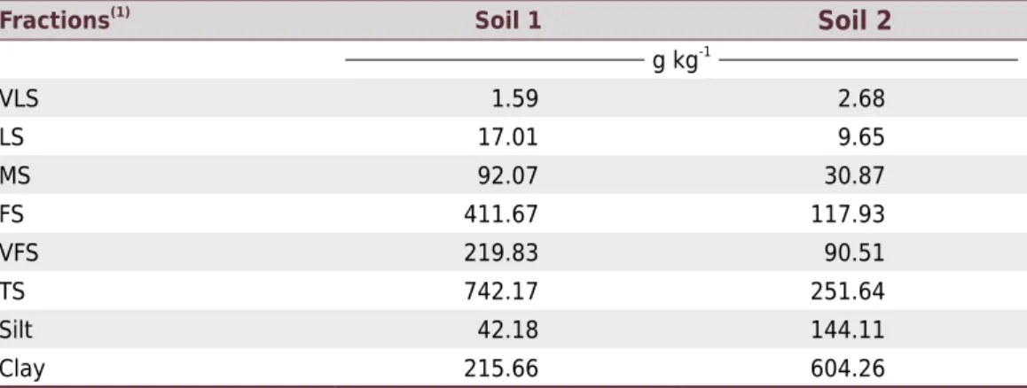
The disturbed samples of each soil were used to perform the granulometric analysis by the densimeter method (Grossman and Reinsch, 2002), to determine the particle density by the method of a helium gas pycnometer and the organic carbon by the Walkey-Black method. The granulometric distribution, splitting the sand fraction according
to the American classification (1951), is presented in table 1. From this distribution, the diagnostic horizon of soil 1 is classified as a clay-sandy-loam texture and that of soil 2
as a loam-texture (Santos et al., 2013).
The undisturbed soil samples were used to determine the soil bulk density (ρ) and the
retention curves. They were also collected from the depth of 0.50 m in soil 1 and from the depth of 0.30 m in soil 2. The samples were collected with the Uhland extractor, which consists of a “cup” with an internal diameter of 75 and height of 75 mm. Rings of
internal diameter of 70 mm, and three different heights, 75 mm (S1), 50 mm (S2), and
25 mm (S3), were used. For the two smaller rings (S2 and S3), the internal space of the “cup” not occupied by the ring wall was completed with extra rings. For S2, two rings of 12.5 mm were used and, for S3, two rings of the same height (25 mm) were used,
Table 1. Granulometric distribution of the diagnostic horizon of the studied soils
Fractions(1) Soil 1
Soil 2 g kg-1
VLS 1.59 2.68
LS 17.01 9.65
MS 92.07 30.87
FS 411.67 117.93
VFS 219.83 90.51
TS 742.17 251.64
Silt 42.18 144.11
Clay 215.66 604.26
VLS = very large sand; LS = large sand; MS = medium sand; FS = fine sand; VFS = very fine sand; TS = total sand; Soil 1 = Typic Hapludox; Soil 2 = Kandiudalfic Eutrudox. (1)
in such a way that the main rings, that is, those that were used in the analyses, were located in the central part of the extractor. A total of 135 samples were collected from each soil: 45 for each sample height.
After collection, the excess of soil in the main rings was removed by taking off the extra rings from S2 and S3, so that the soil would fill the main ring. Then, at one end of the main ring, a fabric was fixed with an elastic to prevent loss of soil during handling of the samples.
The soil water retention curves were determined in the laboratory using porous plate funnels and Richards pressure chambers (Klute, 1986). The tension applied to the funnels was 0.5, 1, 4, 6, and 10 kPa and in the chambers the tensions were 33, 100,
and 500 kPa. Each point of the curve was obtained with five samples for each point.
It was decided to detail the wet part of the curve (points 0.5 to 10 kPa) because the soil
structural arrangement has more influence on the water retention in the wet part of the
curve (lower tension points), where the capillarity is more active.
The samples were saturated for 24 h with distilled and deaerated water and then taken to the funnels, which also had their plates saturated for the same period of time. After the samples were placed in the funnel, the water level was raised above the porous plate to the top of the sample, to ensure saturation of the sample. With the chambers, the saturation of the samples was also for 24 h while the porous plates were immersed in a container with water and only removed when they were used. After the saturation, the samples were taken to the plates, always being careful to ensure perfect plate/sample contact. Then, suction was applied in the case of the funnels, and air pressure in the case of the chambers, corresponding to the desired tension. This caused the soil solution to
drain from the sample until equilibrium was reached when the flow of water stopped, and the matric potential off set the suction (h) or the air pressure (P).
At equilibrium, the samples were removed from the chambers and funnels and weighed in an analytical balance with a hundredth of gram precision and their masses recorded; then they were placed in a forced air circulation oven at 105 °C for two days; after this period, the samples were weighed again and the mass-based and volume-based water contents were then calculated.
The water content data for each tension were fitted to the equation 1, used by van
Genuchten (1980):
θ = θr+ θs ‒ θr
[1 + (α |ϕm| n
]m Eq. 1
In which θs is the saturated soil water content (m
3 m-3), θ
r is the residual soil water
content (m3 m-3), ϕ
m is the matric potential (tension |ϕm|), α, n, and m are parameters
of the equation, with m = 1- 1/n. Both θs and θr were considered as fit parameters and
their values represent the maximum and minimum limits of the curve, respectively. The
parameters α and n are shape parameters related to the pore-size distribution.
The soil pore-size distribution was done using the model that uses the retention curve
and the capillary theory (Libardi, 2012). The pore classification used was that suggested by Koorevaar et al. (1983), in which pores with radius smaller than 15 μm (equivalent to 10 kPa) are micropores, those with radius between 15 and 50 μm (between 3 and 10 kPa) are mesopores, and those larger than 50 μm (equivalent to 3 kPa) are macropores. For application of the soil pore-size distribution model, equation 1 was modified by replacing |ϕm| by the radius of the equivalent pore (r) using the Laplace equation of
capillarity with a contact angle equal to zero. Thus, equation 1 becomes equation 2:
θ = θr+ θs ‒ θr
1 + A nm r
in which
A = 2σα103 Eq. 3
kPa-1 being the unit of α; μm the unit of
r; and kN m-1 the unit of the surface tension of
water σ.
By the differentiation of equation 2 we obtain equation 4, calculating dθ/dlogr. And with the derivative of equation 4 equal to zero, we obtained the equivalent porous radius
(rmax) value corresponding to the máximum value of dθ/dlogr (Equation 5):
= (θs- θr ) mnAnr‒n [1+ Anr‒n]‒m‒1 dθ
dlogr Eq. 4
rmax =A 1 ‒ m
1
n Eq. 5
The data of macro, meso, and microporosity obtained from the soil pore size distribution for each studied sample were submitted to the Shapiro–Wilk parametric normality test, in order to verify if the results were from a population with normal distribution. Then, a comparison of means (Tukey at 0.05 %) was performed using the analysis of variance
to determine if there was any modification in the porosity of the samples when using different heights.
The fitting of data to equation 1 was done with the help of the Table Curve 2D (SPSS Inc., 2000). To verify whether or not there was a difference between the retention curves for the different heights of sample, confidence intervals were plotted to the curves for the
three sample heights in each studied soil.
RESULTS AND DISCUSSION
The clay fraction decisively determines the physical behavior of the soil, due to its
high specific surface area that directly interferes in the soil water retention, because
the surfaces of the clays are negatively charged and adsorb large amounts of water
molecules to the soil surface. Soil 2 (Kandiudalfic Eutrudox), with a very clayey textural classification, may have a higher amount of intra-aggregate pores, high specific surface area, and higher total porosity (α) and, therefore, lower soil bulk density, whereas soil 1
(Typic Hapludox), because it is more sandy, presents a smaller total porous space and, therefore, a higher bulk density (Table 2).
According to the analysis of variance (ANOVA) carried out for the bulk density of the
soil 1 and soil 2 samples, there was no statistical difference between the means of bulk density due to the difference in height of the samples in the two soils. This proves that the sampling in rings of different heights did not cause significant differences of bulk
density. It was also observed that the use of the Uhland extractor with the extra rings in the samples S2 (50 mm high) and S3 (25 mm high) contributed to the minimum
Table 2. Clay fraction, organic carbon, bulk density, particle density and total porosity of the
studied soils
Soils Clay(1) OC(2) ρ(3) ρs (4)
α(5) g kg-1
Mg m-3
m3 m-3
Soil 1 215.66 2.35 1.51 2.67 0.43
Soil 2 604.26 7.46 1.33 2.89 0.54
OC = organic carbon; ρ= bulk density; ρs= particle density; α = total porosity; Soil 1 = Typic Hapludox;
Soil 2 = Kandiudalfic Eutrudox. (1)
Densimeter method; (2)
Walkey-Black method; (3)
Volumetric ring method;
(4)
disturbance of the samples at the moment of sampling and also that to collect an undisturbed soil sample with a ring height less than 25 mm using this extractor would certainly compromise the structure of this sample.
Before discussing the result of the retention curves, it is necessary to remember that, by the theory of the method of determining the retention curve by means of the funnels and pressure chambers with porous plates, the sample height should be as small as possible
to avoid the influence of gravity. This can be illustrated considering figure 1, which shows
a porous plate funnel with a soil sample of height L under a tension h at its base. Consider
points 1 (top) and 2 (base) of the soil sample and the water in equilibrium. By the theory
of potentials, the total water potential in 1 (ϕt1) equals the total water potential in 2 (ϕt2),
that is, ϕt1 = ϕt2. Since ϕt = ϕg+ϕm, ϕg being the gravitational potential, then ϕg1 + ϕm1 = ϕg2 + ϕm2 or, from figure 1, L + ϕm1 = 0 – h and, therefore, ϕm1 = - (h + L), which shows
that the greater L (the height of the sample), the lower the soil water matric potential (or the higher the soil water tension). As the soil water content in the retention curve normally decreases with the increase of the soil water tension, then, the higher L, the lower should be the soil water content in the sample as a whole, mainly for low tensions.
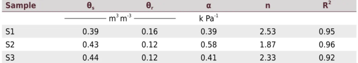
The fitting parameters of the experimental data to equation 1 (van Genuchten, 1980) is presented in table 3. Soil 1 had a saturated soil water content (θs) of 0.39 m3 m-3 for
the 75 mm sample height; 0.43 m3 m-3 for the 50 mm sample height and 0.44 m3 m-3 for
the sample height of 25 mm; that is, θs increased with the decrease of the sample size. The residual soil water content (θr) varied between 0.16 and 0.12 m
3 m-3, with smaller
values for samples of smaller size.
P atm
P atm 1
2 L RG
h
Figure 1. Funnel of porous plate with a sample under a tension h. Patm = atmospheric pressure;
L = height of the sample; RG = gravitational reference; h = suction (tension) (Libardi, 2012).
Table 3. Parameters of the soil 1 (Typic Hapludox) retention curves with samples S1, S2, and S3
Sample θs θr α n R2
m3 m-3
k Pa-1
S1 0.39 0.16 0.39 2.53 0.95
S2 0.43 0.12 0.58 1.87 0.96
S3 0.44 0.12 0.41 2.33 0.92
θs = saturated water content; θr = residual water content; α and n = parameters of the equation; R2 = coefficient
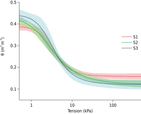
The colorful shadow around each mean retention curve (red curve S1 - 75 mm high; green curve S2 - 50 mm high; blue curve S3 - 25 mm high) of soil 1 (Figure 2) represents
the confidence interval, which permits us to say if the curves are or are not different. The curve S1 (red) was different only from the curve S3 (blue) in the 0-1 kPa range of tension, and in its drier final part it was different from S2 and S3, between the tensions
of 100 and 500 kPa (Figure 2). These higher water content values for the higher tensions
of S1 are probably due to the higher soil volume of these samples, with the fine and very fine sand particles representing 85 % of the total sand fraction, which might have offered more resistance to the air pressure in the water withdrawal from S1 samples of
soil 1. The smaller soil water content values in the initial part of the S1 curve (tension
<1kPa) should be related to the smaller value of θs in the 75 mm sample, caused by gravity as explained in figure 1.
Sandy soils shows high resistance to modification of their structure, for example,
Cubilla et al. (2002) found that there was no change in the bulk density of a sandy-loam
soil under different soil and plant management. Several studies in soils of the state of São Paulo, found that water retention was positively influenced by the clay content in cultivated soils and that in soil under forest, water retention at different depths was
dependent on the organic matter content (Grohmann and Medina, 1962).
From the retention curves of soil 2 (Kandiudalfic Eutrudox) shown in figure 3 and the values of the fit parameters (θs, θr, α, and n) in table 4, it is possible to observe that the larger the sample height, the lower the water content at low tensions, i.e., S3 > S2 ≥ S1. The S1 and S2
curves show lower soil water content in the initial part of the curve, mainly until the tension
of 10 kPa, in which data were obtained using the Haines funnel. The S3 curve is significantly different in relation to the S1 and S2 curves, until near the tension of 10 kPa, since there is no intersection between the confidence interval obtained for S3 (blue) and the confidence intervals of S1 and S2 (red and green). Thus, the height of the sample influenced in a more
remarkable way the soil water retention curvesof soil 2 than those of soil 1.
As already mentioned, it is known from the theory of the method of determination of the retention curve by the funnels and pressure chambers with porous plate, that the soil
sample height should be as small as possible to avoid any influence of the gravitational
S1 S2 S3
Tension (kPa) 1
0.1 0.2 0.3 0.4 0.5
θ (m
3 m -3 )
10 100
Figure 2. Retention curves and confidence intervals obtained with samples S1 (75 mm), S2
potential. However, the sample must be extracted from the soil with such a height that the extraction does not damage the soil structure and interfere in the maintenance of the connection between its own pores and between its pores and the pores of the plate. In other
words, any factor that influences the structural organization of the sample will affect the
water content measured at each tension (Beutler et al., 2002), especially at the beginning of the curve (lower tensions), where the capillary forces are more active. Changes were observed in soil structure caused by the use and management of soil altering considerably the shape of the retention curves, with a reduction of soil porosity and alteration of the soil
pore diameter distribution (Klein and Libardi, 2002). The differences observed in the soil structure can also be attributed to soil mineral particles, which influence the aggregation
processes, the structural arrangement, the total pore volume, and the distribution, as well as the connectivity among poresand tortuosity (Lu et al., 2014).
From the percolation theory, Larson and Morrow (1981) have shown that more representative results can be obtained by reducing the sample size, for the applied tensions, and also for the pore size distribution. Moreover, these authors also stated that the retention curve
is influenced not only by the pore wetting properties and pore geometry, but also by
pore accessibility, facts that are sensitive to the size of the sample used in the analyses.
Differences in retention curves also were found due to the effect of the sample size by Zhou and Stenby (1993). In the case of soil 2, the effect of gravity was more pronounced than in soil 1, leading to a significant difference of the retention curves at low tensions,
between the 75 mm and the 25 mm sample heights, probably because of its structure allowing a greater drainage through the larger or interaggregated pores, a fact that did not occur with the same intensity in soil 1, whose structure is massive.
Figure 3. Retention curves and confidence intervals obtained with samples S1 (75 mm), S2
(50 mm), and S3 (25 mm), in soil 2 (Kandiudalfic Eutrudox).
S1 S2 S3
Tension (kPa) 1
0.35 0.40 0.50 0.55 0.60
θ (m
3 m -3 )
10 100
0.45
Table 4. Parameters of the soil 2 (Kandiualfic Eutrudox) retention curves with samples S1, S2 and S3
Sample θs θr α n R
2
m3 m-3 k Pa-1
S1 0.47 0.35 1.04 2.59 0.91
S2 0.47 0.34 0.81 1.85 0.80
S3 0.59 0.35 0.70 1.94 0.95
θs = saturated water content; θr = residual water content; α and n = parameters of the equation; R2 = coefficient
The soil pore-size distribution constitutes important information to verify the soil pore geometry in the undisturbed soil samples used to determine the retention curve. The
pore radius frequency curves of soil 1 (Figure 4) did not show differences for the different
heights of the sample. The peak of the S2 curve (dotted curve) is a little shifted to the right in relation to the peak of curves S1 and S2, which were coincident for the same
radius (40 μm); and in curve S3 (dashed curve) the radius of the maximum frequency
of the pores (the height of the peak) was higher than the other curves.
Being sandy, this soil contributes to a more uniform structural organization, so that the
difference among the curves may be linked to other factors and not only to the size of the undisturbed sample. In studying the influence of the sand fraction on water retention
and water availability in soils originated from sandstone, Fidalski et al. (2013) found that
fine sand was responsible for the formation of smaller pores and greater retention of
water when compared to another soil of more sandy texture. The soil pore distribution depends on the combination of soil texture and soil structure: the pores due to the texture (ultra and cryptomicropores) strongly retain the water in the soil by adsorption, and the secondary pores, that is, the structural ones, correspond to the spaces within
the soil aggregates (Zaffar and Lu, 2015).
For soil 1, there was no statistical difference between the mean values of the macro and mesopore percentage (Figure 5) when using samples of different heights to determine
the retention curve. Only in the S3 sample there was a decrease of the percentage of micropores when compared to the other samples. As already noted, this must be related
to the greater difficulty of the higher samples to allow water withdrawal at higher tensions
due to the greater resistance to the air pressure in the air chamber.
In the pore radius frequency curves of soil 2 (Figure 6) it is possible to verify that the
distribution of the pores was different: with a solid curve for S1, dotted curve for S2,
and dashed for S3.
The maximum radius frequency per unit of the logarithm of radius of the curves, obtained by equation 5, did not coincide and there was a considerable amplitude of the pore radius frequencies between the curves, i.e., the model overestimates the most frequent radius. This happened because soil 2 presents a very clayey texture and a very developed and
quite complex structure. Due to this structural complexity, many aspects can influence
the frequency of pore distribution in this soil. In this study, the samples with 75 mm and 50 mm heights (S1 and S2) were those that presented a greater facility to drain water when submitted mainly to the suction in the porous plate funnels. This probably occurs through the increase of gravitational potential in these samples due to the greater height above the point at which the measurements were made (porous plate), leading
consequently to the differences in the frequency curves of the pore radius. Therefore,
evidently, the smaller the height of the sample used to determine the retention curve,
the lower the influence of this factor on the soil pore distribution.
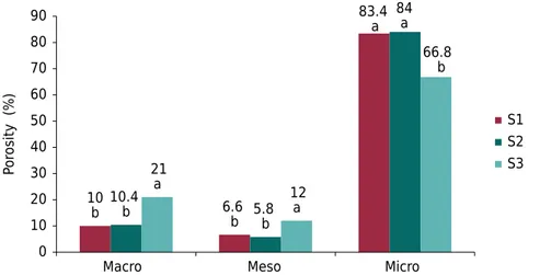
Statistical differences were verified for macro, meso, and micropores when sample S3
(white column) was used, whereas for S1 (black column) and S2 (gray column) there
was no difference (Figure 7). It can also be seen that the percentage of micropores in
S1 and S2 was greater than in S3, the inverse occurring with the percentage of meso and macropores.
The results and the methodology of determination of the retention curve used in this work lead to the recommendation to use undisturbed soil samples with a height of 25 mm. This is because a) experimentally, undisturbed soil samples collected with a height of 25 mm did not compromise its structure, the same not being true of samples smaller than 25 mm, and b) from the results of this work, with samples larger than 25 mm, especially for well structured soils, the values of water content in the wet part of the
21.6 a
29.8 a
48.6 a
29.6 a
23.4 a
46.2 ab
27.6 a
33 a
39.4 b
0 10 20 30 40 50 60
Macro Meso Micro
Po
ro
sity (%
)
S1 S2 S3
Figure 5. Mean values of macropores, mesopores, and micropores obtained with samples S1
(75 mm), S2 (50 mm), and S3 (25 mm) in soil 1 (Typic Hapludox).
0 0.06 0.12
0.1 1 10 100 1000
Radius (μm)
S1 S2 S3
dθ/dlog(r)
Figure 6. Radius frequency function curves for soil 2 (Kandiudalfic Eutrudox), S1 (75 mm),
S2 (50 mm), and S3 (25 mm). 0 0.06 0.12 0.18
0.1 1 10 100 1000
dθ/dlog(r)
Radius (μm)
S1 S2 S3
Figure 4. Radius frequency function curves for soil 1 (Typic Hapludox), S1 (75 mm), S2 (50 mm),
CONCLUSION
The process of the extraction of undisturbed soil samples of small height by means of the traditional Uhland extractor, with rings subdivided into three parts and using the central part to determine the retention curve, proved to be adequate and, with it: i) the retention curve of soil 1 (Typic Hapludox) determined with samples of height 25 mm was
different from that determined with samples of height 75 mm, for the 0-1 kPa range of tension, and different from those determined with samples of heights 50 and 75 mm, for the tension range 100-500 kPa; ii) for soil 2 (Kandiudalfic Eutrudox), the retention curve with samples of 75 mm height was very different, both in relation to the curve
with samples of 50 mm height and in relation to that with samples of 25 mm height, in the 0-10 kPa range of water tension.The pore-size distribution curves for the three
sample heights were very different for soil 2 and slightly different for soil 1. In view of these findings and the fact that the sample must have the smallest possible height, it is
recommended to use undisturbed soil samples with a height of 25 mm.
REFERENCES
Abbasi F, Javaux M, Vanclooster M, Feyen J. Estimating hysteresis in the soil water retention curve from monolith experiments. Geoderma. 2012;189-190:480-90. https://doi.org/10.1016/j.geoderma.2012.06.013
Beutler AN, Centurion JF, Souza ZM, Andrioli I, Roque CG. Retenção de água em dois tipos de Latossolos sob diferentes usos. Rev Bras Cienc Solo. 2002;26:829-34. https://doi.org/10.1590/S0100-06832002000300029
Bittelli M, Flury M. Errors in water retention curves determined with pressure plates. Soil Sci Soc Am J. 2009;73:1453-60. https://doi.org/10.2136/sssaj2008.0082
Brito AS, Libardi PL, Mota JCA, Moraes SO. Estimativa da capacidade de campo pela curva
de retenção e pela densidade de fluxo da água. Rev Bras Cienc Solo. 2011;35:1939-48.
https://doi.org/10.1590/S0100-06832011000600010
Burdine NT. Relative permeability calculations from pore size distribution data. J Petrol Technol. 1953;5:71-8. https://doi.org/10.2118/225-G
Claessen MEC. Manual de métodos de análise de solo. 2. ed. Rio de Janeiro: Embrapa Solos; 1997.
Cooper M, Vidal-Torrado P, Lepsh IF. Stratigraphical discontinuities, tropical landscape evolution and soil distribution relationships in a case study in SE-Brazil. Rev Bras Cienc Solo. 2002;26:673-83. https://doi.org/10.1590/S0100-06832002000300012
10
b 6.6
b
83.4 a
10.4
b 5.8
b
84 a
21 a
12 a
66.8 b
0 10 20 30 40 50 60 70 80 90
Macro Meso Micro
Po
ro
sity (%)
S1 S2 S3
Figure 7. Mean values of macropores, mesopores and micropores obtained with samples S1
Cubilla M, Reinert DJ, Aita C, Reichert JM. Plantas de cobertura do solo: uma alternativa para aliviar a compactação em sistema plantio direto. Revista Plantio Direto. 2002;71:29-32.
Fidalski J, Tormena CA, Alves SJ, Auler PAM. Influência das frações de areia na retenção e disponibilidade de água em solos das formações Caiuá e Paravanaí. Rev Bras Cienc Solo.
2013;32:613-21. https://doi.org/10.1590/S0100-06832013000300007
Ghanbarian B, Taslimitehrani V, Dong G, Pachepsky YA. Sample dimensions effect on prediction
of soil water retention curve and saturated hydraulic conductivity. J Hydrol. 2015;528:127-37. https://doi.org/10.1016/j.jhydrol.2015.06.024
Grohmann F, Medina HP. Características de umidade dos principais solos do estado de São
Paulo. Bragantia. 1962;21:285-95. https://doi.org/10.1590/S0006-87051962000100018
Grossman RB, Reinsch TG. Bulk density and linear extensibility. In: Dane JH, Topp CG, editors. Methods of soil analysis: Physical methods. 3rd ed. Madison: Soil Science Society of America; 2002. Pt. 4. p. 201-28.
Hunt AG, Ewing RP, Horton R. What’s wrong with soil physics? Soil Sci Soc Am J. 2013;77:1877-87. https://doi.org/10.2136/sssaj2013.01.0020
Hunt AG, Skinner TE. Hydrolic condutivity limited equilibartion: effect on water-retention
caracteristics. Vadose Zone J. 2005;4:145-50. https://doi.org/10.2136/vzj2005.0145
Klein VA, Libardi PL. Densidade e distribuição do diâmetro dos poros de um Latossolo vermelho, sob diferentes sistemas de uso e manejo. Rev Bras Cienc Solo. 2002;26:857-67. https://doi.org/10.1590/S0100-06832002000400003
Klute A. Water retention: laboratory methods. In: Klute A, editor. Methods of soil analysis: Physical and mineralogical methods. 2nd ed. Madison: American Society of Agronomy, Soil Society of America; 1986. Pt. 1. p. 635-62.
Koorevaar P, Menelik G, Dirksen C. Elements of soil physics. Amsterdan: Elsevier; 1983.
Larson RG, Morrow NR. Effects of sample-size on capillary pressures in porous media. Powder
Technol. 1981;30:123-38. https://doi.org/10.1016/0032-5910(81)80005-8
Libardi PL. Dinâmica da água no solo. 2. ed. São Paulo: Editora da Universidade de São Paulo; 2012.
Lu S-G, Sun F-F, Zong Y-T. Effect of rice husk biochar and coal fly ash on some
physical properties of expansive clayey soil (Vertisol). Catena. 2014;114:37-44. https://doi.org/10.1016/j.catena.2013.10.014
Machado JL, Tormena CA, Fidalski J, Scapim CA. Inter-relações entre as propriedades físicas e os coeficientes da curva de retenção de água de um Latossolo sob diferentes sistemas de uso. Rev
Bras Cienc Solo. 2008;32:495-502. https://doi.org/10.1590/S0100-06832008000200004
Moraes SO, Libardi PL, Dourado Neto D. Problemas metodológicos na obtenção da curva de retenção da água pelo solo. Sci Agric. 1993;50:383-92. https://doi.org/10.1590/S0103-90161993000300010
Mualem Y. A new model for predicting hydraulic conductivity of unsaturated porous media. Water Resour Res. 1976;12:513-22. https://doi.org/10.1029/WR012i003p00513
Munoz-Carpena R, Regalado CM, Alvarez-Benedi J, Bartoli F. Field evaluation of the new philip-dunne permeameter for mensuring saturated hydraulic conductivity. Soil Sci. 2002;167:9-24. https://doi.org/10.1097/00010694-200201000-00002
Reichardt K, Timm LC. Solo, planta e atmosfera: conceintos, processos e aplicações. 2. ed. São
Paulo: Editora Manole; 2004.
Santos HG, Jacomine PKT, Anjos LHC, Oliveira VA, Oliveira JB, Coelho MR, Lumbreras JF, Cunha TJF.
Sistema brasileiro de classificação de solos. 3. ed. rev. ampl. Rio de Janeiro: Embrapa Solos; 2013. Soil Survey Staff. Keys to soil taxonomy. 12th ed. Washington, DC: United States Department of
Agriculture, Natural Resources Conservation Service; 2014.
Solone R, Bittelli M, Tomei F, Morari F. Errors in water retention curves determined
with pressure plates: effects on the soil water balance. J Hydrol. 2012;470-471:65-74.
SPSS Inc. Table curve 2D: automated curve fitting and equation discovery. Chicago, SPSS
Science; 2000.
van Genuchten MT. A closed-form equation for predicting the hydraulic conductivity of unsaturated soils. Soil Sci Soc Am J. 1980;44:892-8. https://doi.org/10.2136/sssaj1980.03615995004400050002x
Zaffar M, Lu SG. Pore size distribution of clayey soils and its correlation with soil organic matter.
Pedosphere. 2015;25:240-9. https://doi.org/10.1016/S1002-0160(15)60009-1