Static Limit Analysis of Reinforced Soil Structures by a Simple Finite Element and Second-Order Cone Programming

Abstract

To discretize reinforced soil structures in plane strain and predict their collapse load, a simple three-node triangular finite element is formulated based on the static theorem of the limit analysis. The element satisfies the equilibrium equations and the mechanical boundary conditions in a weak sense. A modified Mohr-Coulomb yield surface is adopted to describe the reinforced soil behavior from a macromechanics point of view. It is also taken into account the possibility of tension failure of the reinforcement and failure of the reinforcement interface. The stated nonlinear convex optimization problem is cast as second-order cone programming. Numerical exam-ples illustrate the predictive accuracy of the above scheme as well as the efficiency and speed of an interior-point method to reach optimal solutions.

Keywords

reinforced soil; static theorem; finite element; second-order cone programming

Static Limit Analysis of Reinforced Soil Structures by a Simple

Finite Element and Second-Order Cone Programming

1 INTRODUCTION

In the design of reinforced soil structures, the maximum load to be resisted at the impending collapse must be evaluated. The ability of the methods to accurately estimate ultimate limit states depends on the fulfillment of theoretical requirements derived from continuum mechanics concerning the equi-librium, strain-displacement relations, constitutive behavior and boundary conditions. Under certain restrictions, the theory of plasticity allows the prediction of the collapse load by means of the limit analysis based on the bound theorems (Drucker et al._{, 1952). Numerical solutions are most facilitated}

Eric Luis Barroso Cavalcante a,* Eliseu Lucena Neto b

Denilson José Ribeiro Sodré c

a _{Tribunal de Contas da União,} 70042-900 Brasília, DF, Brazil.

ericlb@tcu.gov.br

b _{Instituto Tecnológico de Aeronáutica,} 12228-900 São José dos Campos, SP, Brazil. eliseu@ita.br

c _{Universidade Federal do Pará,} 66075-110 Belém, PA, Brazil dsodre@ufpa.br

*_{Corresponding author}

http://dx.doi.org/10.1590/1679-78253745 Received 05.02.2017

in this case coupling such theorems with the finite element method, as originally proposed by Lysmer (1970) and Bottero et al. _{(1980). This is a straightforward approach for computing lower and upper}

bounds on the load at incipient collapse which have gained increasing attention (Lyamin and Sloan, 2002; Krabbenhoft and Damkilde, 2003; Makrodimopoulos and Martin, 2006; Yu and Tin-Loi, 2006; Ciria et al._{, 2008; Munõz} et al._{, 2009; Le} et al._{, 2010; Bleyer and de Buhan, 2014; Nguyen-Thoi} et al._,

2015). This is partly due to the development of robust optimization methods and solvers on which they strongly rely (Drud, 1996; Sturm, 1999; Lyamin and Sloan, 2002; Murtagh and Saunders, 2003; Tütüncü et al._{, 2003; Andersen} et al._{, 2003; Krabbenhoft and Damkilde, 2003).}

The identification of failure modes through experiments has had an essential impact on the de-velopment of reinforced soil mechanics. It has been realized that, in the case of sufficiently good bonding between soil and reinforcement, reinforced soil behaves, in the macroscopic scale, like a ho-mogeneous material. This important observation was confirmed by laboratory investigations reported in Long et al. _{(1972) and Chapuis (1980). Reinforced soil can then be treated as a composite material}

formed by the association of frictional soil and tension-resistant fiber elements, such as geosynthetics, with behavior presumed homogeneous and anisotropic from a macromechanics point of view. The material strength is estimated from the strength characteristics of its components and the interaction between them. Limit analysis procedures derived from the referred macromechanics approach have been successfully applied to predict the observed response of reinforced superficial foundations and earth walls (Sawicki, 1983; Kulczykowski, 1985; Sawicki and Lesniewska, 1987, 1989; de Buhan et al_.,

1989; de Buhan and Siad, 1989; Yu and Sloan, 1997).

In this paper, specific attention is focused on the static approach of the limit analysis coupled with the finite element method to provide limit load solutions for reinforced soil structures in plane strain. In the description of the soil behavior, the isotropic Mohr-Coulomb yield surface is modified to include the effect of anisotropy caused by the presence of reinforcement. It is also taken into account the possibility of tension failure of the reinforcement and failure of the soil-reinforcement interface (de Buhan and Siad, 1989). The finite element proposed for limit analysis, which has its roots in the classic paper by Anderheggen and Knöpfel (1972), satisfies the equilibrium equations and the mechanical boundary conditions on average. In this sense, a solution obtained with this weak equilibrium model is not a strict lower bound. The formulation of the static theorem is then written within the framework of a nonlinear convex optimization technique, known as second-order cone programming (Lobo et al._{, 1998).}

There is no analytical approach for the solution of general convex optimization problems, but there are very effective methods for solving them (Boyd and Vandenberghe, 2009). The interior-point method employed in this paper works extremely well in practice. It was developed by Andersen et al.

Figure 1: Stresses on reinforced soil.

2 FAILURE CONDITIONS

The reinforced soil in this paper will be treated as a homogeneous composite material with anisotropic properties. The reinforcement is assumed to be unidirectional with thickness d very small compared to the space h between two reinforcements (

d h



1

macrostresses, and tensors s s s s T

t n tn

s s t

ê ú

= ê_ë ú_û

s and r r r r T

t n tn

s s t

ê ú

= ê_ë ú_û

s for microstresses which act on the soil and reinforcement, respectively. The tensor components are related by

s r s r

t t t t

s r

n n n

s r

tn tn tn

d h

s s s s s

s s s

t t t

= + = +

= =

= =

(1)

where r r t

d h

s = s (Yu and Sloan, 1997).

The relations between the macrostress components in the orthogonal Cartesian coordinate sys-tems xy e tn are

(

)

(

)

2 2

2 2

2 2

cos sin 2 sin cos sin cos 2 sin cos

sin cos cos sin

x t n tn

y t n tn

xy t n tn

s s q s q t q q

s s q s q t q q

t s s q q t q q

= +

-= + +

= - +

-(2)

where q represents the angle between the horizontal axis x and the reinforcement direction t, meas-ured counterclockwise. Substitution of (1) and relations

x

t

q

microstresses

sn

t

t

r

st

y

soil

n

sn

t

t

st

x

t

y

n

s

t

ttn

s

q

d

(

)

(

)

2 2

2 2

2 2

cos sin 2 sin cos sin cos 2 sin cos

sin cos cos sin

s s s s

t x y xy

s s s s

n x y xy

s s s s

tn x y xy

s s q s q t q q

s s q s q t q q

t s s q q t q q

= + +

= +

-= - - +

-(3)

into (2) yields

2

2

cos sin

sin cos .

s r x x s r y y s r xy xy

s s s q

s s s q

t t s q q

=

-=

-=

-(4)

The reinforcement inside the soil is supposed to act merely as tensile load carrying elements (de Buhan et al_{., 1989). The bounds}

o

0_£sr _£s

(5)

are thereby imposed on sr, where s_o =

( )

rein-forcement times its volumetric fraction.

The soil mass with cohesion c and angle of internal friction f is initially assumed to obey the

Mohr-Coulomb yield surface in plane strain (Muñoz et al._{, 2009):}

(

) (

)

(

)

2 2 cos sin

s s s s s

s x y xy x y

F = s -s + t -é_êë c f- s +s fù_úû (6)

This expression is then modified to include the effect of anisotropy caused by the presence of reinforcement using relations (4):

(

) (

)

(

)

cos 2 2 sin 2 2 cos sin

r r r

s x y xy x y

F = s -s -s q + t -s q -_êëé c f- s +s -s f_ûù_ú

.

The soil-reinforcement interface failure surface is assumed to be described by

| | tan

i tn i n i

F = t -c +s f ₍₈₎

where ci and fi denote the interface cohesion and angle of internal friction, respectively (Yu and

Sloan, 1997). In view of (2), the failure surface (8) takes the form

(

)

(

)

1

| sin 2 2 cos 2 | sin cos sin 2 tan 0

2

i y x xy i x y xy i

F = s -s q+ t q -c + s q+s q-t q f = ₍₉₎

3 STATIC THEOREM

The limit analysis relies on the assumption of an elastic-perfectly plastic material with a flow rule associated to a convex yield surface, and also on small displacement gradients so that the body does not undergo large deformation at collapse (problem readily stated on the undeformed body geometry). The static approach of the limit analysis requires that the assumed stress field must satisfy the equi-librium equations, the mechanical boundary conditions and the yield criterion everywhere. Under these idealized conditions, the computed limit load is a lower bound on the true collapse load (Chen, 1975).

3.1 Equilibrium Equations

Let W be the region occupied by the reinforced soil structure subjected to the body force

T

x y

b b

ê ú

= ê_ë ú_û

b expressed in the system xy. The macrostress field s_{= ê}ê_ës_x s_y t_xyú_úûT must satisfy the equilibrium equations

+ =0

s

D b (10)

throughout the domain W, where the differential operator

0

0

x y

x x

é ¶ ¶ ù

ê ú

ê_{¶ ¶} ú

= ê _{¶ ¶} ú

ê ú

ê ú

ê ú

ë ¶ ¶ û

D . ₍₁₁₎

3.2 Mechanical Boundary Conditions

Let G be the boundary of the domain W, with unit outward normal vector denoted by

T

x y

n n

ê ú

= êë úû

n . In addition to (10), the macrostress field must also satisfy the mechanical boundary

conditions

= s=

t N t (12)

on the portion G_t of G on which the traction (stress vector) t = ê_ëêt_x t_yú_úûT is prescribed as being t. Matrix

0 0

x y

y x

n n

n n

é ù

ê ú

= ê_ê ú_ú

ë û

N ₍₁₃₎

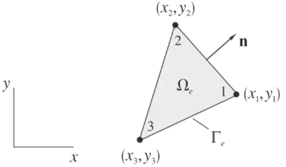
Figure 2: Finite element We with the unit normal vector n on its boundary Ge.

3.3 Yield Criterion

To assure that the yield criterion is satisfied it is necessary to impose simultaneously

o

0 0 0 r

s i

F £ F £ £s £s . ₍₁₄₎

As the function Fi defined in (9) has a term in modulus, the second of inequalities (14) splits

into two other conditions given by

0 1,2

i j x j y j xy i

F =As +Bs +C t -c £ j = ₍₁₅₎

where

2 2

1 1

2

1 2

2

2 2

1 1

sin tan sin 2 cos tan sin 2

2 2

1 sin 2 tan cos 2 sin tan sin 2

2 1

cos tan sin 2 sin 2 tan cos 2 2

i i

i i

i i

A B

C A

B C

q f q q f q

q f q q f q

q f q q f q

= - = +

= - + = +

= - = -

-(16)

4 FINITE ELEMENT FORMULATION

Suppose that the reinforced soil is divided into a number of triangular elements and treated as an assembly of them. To apply the above equations to a typical element W_e shown in Figure 2, the definition of the boundary should be extended to include the traction continuity on the interelement portion G_i:

( )t ++( )t -= 0 ₍₁₇₎

y

x

W

G

n

2

3

1

_{(x ,y )}

1 1

(x ,y )

where the superscripts “+” and “-” denote the two sides of Gi. Expressions (10), (12) and (17) may

now be viewed as the equilibrium within the element and on its boundary G_t and G_i, respectively (Pian and Wu, 2006; Washizu, 1982).

Equations (10), (12) and (17) can be enforced to be satisfied on average over the element and on its boundary by means of

(

)

(

)

e t i

T _{dx dy} T _ds T _ds

W G G

+ - - - =

ò

ò

ò

where w = êê_ëw_x w_yú_úûT is an arbitrary weight function that is continuous on the element domain and

across its interfaces. The last integral when considered jointly with those of the neighborhood elements enforces (17), since it represents one of the terms in ( ) ( ) 0

i

T + - _ds

G

é ₊ ù ₌

ê ú

ë û

ò

In view of the divergence theorem, one writes

(

)

(

)

e e e

T

T _{dx dy} T _ds T _{dx dy}

W G W

=

-ò

ò

ò

where w is additionally assumed to be differentiable once with respect to x and y. Since

e u t i

G = G È G È G , expression (18) is then simplified to

(

)

u t e e

T

T _ds T _ds T _{dx dy} T _{dx dy}

G G W W

+ + - =

ò

ò

ò

ò

where the portion G_u of the element boundary G_e falls on the reinforced soil boundary with pre-scribed displacement.

The macrostress field is linearly approximated over the element by

1 1 2 2 3 3

N N N

= + +

s s s s (21)

where

(

)

1

1,2, 3 2

T

i xi yi xyi Ni i ix iy i

A

s s t a b g

ê ú

= _{êë úû} = + + =

s (22)

are the macrostress nodal values and the shape functions, respectively, with A standing for the triangle area. To evaluate

i x yj k x yk j i yj yk i xk xj

a = - b = - g = - ₍₂₃₎

from the node coordinates, the indices i j k, , should be permuted in a natural order (i¹ j ¹k ).

1 1 2 2 3 3

N N N

= + +

w w w w

,

with nodal values

1,2, 3

T

i = êêëwxi wyiúúû i =

w . (25)

Substitution of (21) and (24) into (20) yields

1 1

2 2

3 3

0 T

ì ü æ ì üö

ï ï _ç ï _ï÷

ï ï _ç ï _ï÷

ï ï _ç ï ï÷

ï ï _{ç -}é ùï ï÷₌ í ý _{ç êë úû}í ý÷_÷

ï ï ç ï ï÷

ï ï ç ï ï÷

ï ï _çè ï ï÷_ø

ï ï ï ï

î þ î þ

s s s

w

w F G G G

w

, (26)

where

2 3 3 2

3 2 2 3

3 1 1 3

1 3 3 1

1 2 2 1

2 1 1 2

1 2 3 1 2 3

0 0 0 1 0 6 0 0 t e T T

y y x x

x x y y

y y x x

x x y y

y y x x

x x y y

ds dx dy

G W

é _{- -} ù

ê ú

ê _{- -} ú

ê ú

ê _{- -} ú

ê ú

= ê _{- -} ú

ê ú

ê _{- -} ú

ê ú

ê _{- -} ú

ê ú

ë û

é ù é ù

=

_ò

_ò

G

F N N N t N N N b

(27) and 0 0 i i i N N é ù ê ú

= ê_ê ú_ú

ë û

N . ₍₂₈₎

Because (26) holds for any arbitrary weight function, it follows that

1 2 3 ì ü ï ï ï ï ï ï ï ï

é ù_{í ý=}

ê ú

ë û ï ï_{ï ï} ï ï ï ï î þ s s s

G G G F . ₍₂₉₎

Elimination of the integral over Gu by choosing w null over there introduces zero components

5 THE SOCP PROBLEM

In the static limit analysis, the structure equilibrium and the yield criterion, expressed in terms of nodal stresses, are constraints of an optimization problem for the applied load maximization. The optimal solution

*

1 2 1 2 o

{max , ( , r) , ( ) , r }

l = l _ls=l_f +_{f g} s s £0 _g s £0 0£s £s ₍₃₀₎

identifies the collapse load, where the applied load has been split into two parts: lf₁ which is adjusted

during the optimization by means of the load factor l, and f₂ which is kept constant. Vectors s

and _sr _{collect the nodal values of s and s}r_{, respectively.}

Under the continuity provided by the approximations (21) and (24), the equality constraint

1 2

l

= +

s

l f f , ₍₃₁₎

which arises from the assembly of (29), represents the discrete equilibrium of the whole reinforced soil structure. The inequalities constraints

1( , ) 2( ) o

r _{£0 £0 0£} r _£

s s s s s

g g ₍₃₂₎

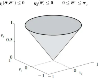
Figure 3: Second-order cone (34).

stem from the evaluation at each node of the first, second and third of inequalities (14), respectively, since it is sufficient to enforce them at each node in order that they are satisfied throughout the mesh. The nonlinear convex optimization problem (30) is not a SOCP problem. To formulate it as such (Lobo et al._{, 1998), we introduce the auxiliary variables}

1 2 3

1 1 0 cos 2 0

0 0 2 sin 2 0

sin sin 0 sin 2 cos 1

x

y

xy r

v v

v c

s s q

t q

f f f f s

ì ü ï ï ï ï ï ï ï ï

ì ü é ù

ï ï - - ï ï

ï ï ê ú ï ï

ï ï _{ï ï}

ï ï ê úï ï

=í ý_{ï ï}= _ê - _úí_ï ý_ï

ê ú

ï ï _{- -} ï ï

ï ï _{ê ú}ï ï

ï ï ï ï

î þ ë _{û ï ï}

ï ï ï ï ï ï î þ

into (7) to state F_s £0 as the three-dimensional second-order cone

2 2

1 2 3 3 0

v +v £v v ³ ₍₃₄₎

sketched in Figure 3. Now, the problem can be treated as SOCP by just replacing _g1( ,_{s s}r)_{£0 with}

1( , , ) 2( ) 3

r _{=0 £0 ³0}

s s

h v h v v ₍₃₅₎

where the vectors v and v₃ collect the nodal values of v and v₃. The new constraints (35) stem from the evaluation of (33) and (34) at each node, and all the problem nonlinearity concentrates in the constraint h₂ £0 related to the cone definition.

The optimization problem solution is carried out following the steps: (a) set up of the SOCP problem with YALMIP (Löfberg, 2004) in the MATLAB environment: problem (30) with g₁£0

replaced by (35); (b) solution by MOSEK using the interior-point optimizer developed for nonlinear convex optimization by Andersen et al_{. (2003).}

6 RESULTS

Predictions of the collapse load for some well-known stability problems of soil mechanics, namely the bearing capacity of footings and the stability of slopes, are computed after the soil is reinforced. This paper focuses on the limit analysis based on the static theorem as well as on the efficiency and speed with which the problems are solved as SOCP. For comparison, the piecewise linearization of F_s

adopted by Yu and Sloan (1997) is accomplished, using 48 sides in the linearized yield polygon pre-sented therein, so that the problems can also be solved as LP by performing a sequence of optimization started with the Newton barrier method and concluded with the simplex method at FICO® Xpress Optimization Suite. The role played by the simplex method in such a procedure is to guarantee that the optimal solution is achieved. The computations are performed on a Sony VAIOTM All-in-One machine (i5 dual core 2.50 GHz CPU, 12 GB RAM), running a 64-bit Windows 7. The reported CPU times refer to the time spent on the optimization iterations.

6.1 Strip Footing on Cohesionless Reinforced Soil

For the strip footing of width B indicated in Figure 4a, only half of the full geometry needs to be considered due to symmetry conditions. To deal with the semi-infinite domain, a rectangular portion is discretized as in Figure 4b extending horizontally from the symmetry plane to the right over a length 3B and vertically downwards to a Depth 2B. This domain is sufficiently extended so that conditions at the far boundary do not have significant effect on the calculated limit load.

In this example, f₁, present in (30), denotes all the loads applied on Gt and f2 =0, also present

0

s

t = on the left (symmetric) edge

0 0

n s

t = t = on the upper edge without strip footing

n

t = -q on the upper edge with strip footing

(36)

where q is the force per unit area exerted by the footing, t_n and t_s are the traction components normal and tangential to the edges.

The weight function components w_n and w_s are imposed to be null at nodes on the edges where the traction components tn and ts are unknown, respectively:

0

n

w = on the left (symmetric) edge

0

s

w = on the upper edge with strip footing. (37)

In addition, w_n and w_s are made to be null on the far right and bottom edges because t_n and

s

t are taken to be unknown over there.

It is well-known that the bearing capacity of strip footing is null when the soil is purely frictional, weightless and subjected to no surcharge (Terzaghi, 1943; Davis and Booker, 1971). The simple in-clusion of horizontal reinforcement, however, rises the bearing capacity to

(

)

e o

1 sin q

e

p _{f f}

f s

æ _ö÷ ç _{+ ÷}

ç ÷

ç ÷

çè ø

= + . (38)

This is the exact solution, as demonstrated by Kulczykowski (1985), when the reinforced soil is treated as a homogeneous and anisotropic composite material with perfectly rough soil-reinforcement interface. Table 1 summarizes our results obtained by simulating the above property using

0

i

c = =c , f_i =f. It is also depicted the number of iterations and the CPU time required to solve the SOCP and the LP problems. The small difference between the SOCP and LP predictions can be reduced increasing the number of sides in the linearized yield polygon. However, the computational cost of an LP solution may become prohibitive for a larger number of sides because of the amount of iterations and CPU time involved. The SOCP number of iterations agrees with already published numerical experiments, in the sense that an interior-point method demands typically between 5 and 50 iterations to solve any SOCP problem (Lobo et al._{, 1998). In the LP solutions, the simplex phase}

answers for 99.2% to 99.9% of the total number of iterations. For instance, out of 10103 iterations for

10

f=  _{the count of 10037 takes place in the simplex phase.}

f SOCP LP

o

q s _{iter CPU} q s_{o iter CPU}

10° 1.3370 36 0.95 1.3362 10103 24 15° 1.8972 30 0.84 1.8953 6864 16 20° 2.5239 37 0.95 2.5210 53023 150 25° 3.4577 40 1.01 3.4511 137467 289 30° 4.8029 26 0.73 4.7904 14094 37 35° 7.0282 33 0.83 7.0000 11473 28 iter: number of iterations CPU: CPU time in seconds

Table 1: Bearing capacity of strip footing on cohesionless reinforced soil.

of the whole domain into triangular elements devised by Lysmer (1970) along with extension elements developed by Pastor (1978). In that work, as stated previously, the optimization problem is conceived as linear programming. For a given mesh, the scheme adopted by Yu and Sloan leads to a much larger problem size because of the use of Lysmer element and the piecewise linearization of F_s. The gap to the exact solution displayed by our predictions is almost steady for all angles of internal friction considered, whereas it is noticeable the deterioration of Yu and Sloan lower bounds for higher values of f.

Figure 5: Strip footing on cohesionless reinforced soil: q soversus f .

6.2 Strip Footing on Cohesive-Frictional Reinforced Soil

The exact bearing capacity of strip footing on weightless unreinforced soil is given by

tan 2

e tan 1 cot

4 2

q =c eêé p f _çç_çæp +fö÷_÷÷- ùú f

÷

ê _{è ø} ú

ë û , (39)

as demonstrated by Prandtl (1920). The advantage of having horizontal reinforcement can be esti-mated by analyzing numerically the change in (39) due to the reinforcement inclusion. The same mesh of Figure 4b is adopted and the mechanical boundary conditions are taken as

10

exact

15

20

25

30

35

1

3

5

7

f

q

s0

present

0

s

t = on the left (symmetric) edge

0 0

n s

t = t = on the upper edge without strip footing

0

n s

t = -q t = on the upper edge with strip footing.

(40)

The weight function component wn is imposed to be null at nodes on the left edge, and wn and

s

w are made to be null on the far right and bottom edges as before.

Table 2 presents the ratio q q_{r e} between the bearing capacities of strip footing on reinforced and

unreinforced soil for different s_o c and angles of internal friction. It is assumed perfectly rough soil-reinforcement interface (c_i =c, f_i =f). Although the SOCP and LP results differ from each other by a small amount, the difference of iterations and CPU time between both optimization techniques is remarkably large. Results for s_o c = 0 illustrate the accuracy of our predictions for the bearing capacity of strip footing on unreinforced soil.

o c

s _f=10 _{f =20} _{f =30}

r e

q q iter CPU q qr e iter CPU q qr e iter CPU

0.0 1.0002† 20 0.67 0.9989 22 0.70 0.9789 21 0.67 0.9980‡ 2683 5 0.9959 2171 3 0.9742 2489 4 0.5 1.0956 23 0.78 1.0896 28 0.78 1.0572 26 0.75

1.0935 3192 5 1.0865 2090 3 1.0521 5394 8 1.0 1.1908 23 0.70 1.1802 27 0.78 1.1350 24 0.72

1.1887 4268 7 1.1770 2573 3 1.1301 4888 8 1.5 1.2859 23 0.72 1.2707 26 0.75 1.2125 24 0.72

1.2838 4248 7 1.2674 2647 4 1.2073 6519 11 2.0 1.3808 22 0.69 1.3611 25 0.73 1.2896 23 0.73

1.3788 3380 6 1.3577 2587 4 1.2842 4585 8 iter: number of iterations CPU: CPU time in seconds †_SOCP ‡_LP

Table 2: Ratio q q_{r e} between the bearing capacities of strip footing on cohesive-frictional soil.

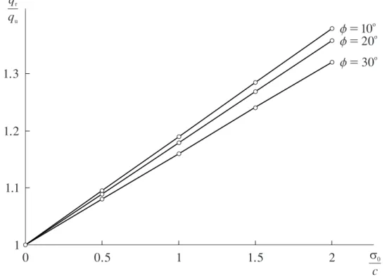
Figure 6 shows the bearing capacity ratio q q_{r u} obtained with SOCP, where q_u refers to the unreinforced scenario. For a given f, the advantage of the reinforcement increases with s_o c. Indeed, the ratio q q_{r u} rises almost linearly with s_o c, where s_o can be augmented by either increasing the reinforcement yield strength s_yield or the reinforcement volumetric fraction d h. We can observe

Figure 6: Strip footing on cohesive-frictional soil: q qr uversus so c for different angles of internal friction f .

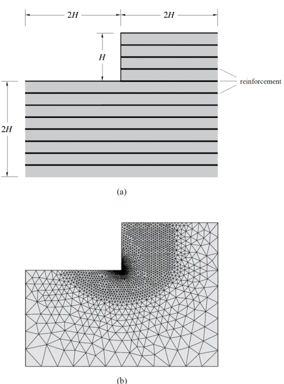
6.3 Cohesionless Reinforced Earth Wall

To deal with the reinforced earth wall, the dimensions depicted in Figure 7a are considered sufficiently large to represent adequately the semi-infinite domain and the mesh adopted in the analysis is shown in Figure 7b. In this example, f₁, present in (30), represents the vertical body force and _f2 =0, also

present in (30), accounts for the null loads acting on G_t. The mechanical boundary conditions are

0 0

n s

t = t = on the three free edges. ₍₄₁₎

On the far left, right and bottom edges, where tn and ts are supposed to be unknown, wn and

s

w are set equal to zero.

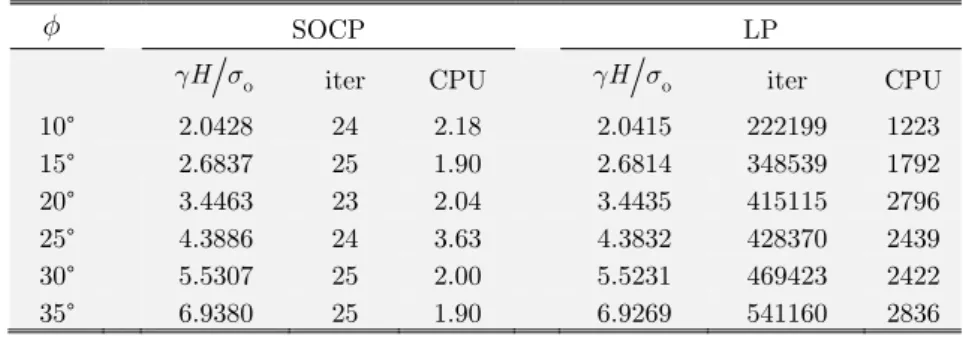
Table 3 condenses our results for horizontal reinforcement under perfectly rough soil-reinforce-ment interface (c_i = =c 0, f_i =f). Note again the small difference between SOCP and LP predic-tions, but a much higher computational cost of an LP solution. Figure 8 shows that our results obtained with SOCP are bracketed by the lower bounds of Yu and Sloan (1997) and the upper bounds

upper 2

o

2 tan

4 2 H

g _{p f}

s

æ _ö÷ ç

= ç_ç + ÷_÷÷

è ø (42)

0.5

1

1.5

2

0

1

1.1

1.2

1.3

s

c

q

q

f

=10

f

=20

of Sawicki and Lesniewska (1987).

f SOCP LP

o

H

g s iter CPU gH so iter CPU

10° 2.0428 24 2.18 2.0415 222199 1223 15° 2.6837 25 1.90 2.6814 348539 1792 20° 3.4463 23 2.04 3.4435 415115 2796 25° 4.3886 24 3.63 4.3832 428370 2439 30° 5.5307 25 2.00 5.5231 469423 2422 35° 6.9380 25 1.90 6.9269 541160 2836 iter: number of iterations CPU: CPU time in seconds

Table 3: Critical height of cohesionless reinforced earth wall.

Figure 8: Cohesionless reinforced earth wall: gH s_o versus f .

6.4 Cohesive-Frictional Reinforced Earth Wall

To estimate the advantage of having horizontal reinforcement in cohesive-frictional earth walls, anal-yses are performed for cases with and without reinforcement. The same mesh and boundary conditions of the previous example are considered. Assuming perfectly rough soil-reinforcement interface (ci =c, fi =f), Table 4 presents the ratio Hr Hc between the critical heights of reinforced and

unreinforced earth wall for different s_o c and angles of internal friction. The values H_c are elaborate upper bounds computed by Chen (1975) for the unreinforced soil using a logarithmic spiral surface discontinuity mechanism passing through the vertical slope toe. Although the difference between the SOCP and LP solutions is small, the computational cost of one technique differs excessively from the

10

15

20

25

30

35

f

1

3

5

7

g

H

s

upper

present

other. Results for s_o c = 0 illustrate that our solutions and Chen upper bounds are in close agree-ment.

o c

s f=10 f =20 f=30

r c

H H _{iter CPU} H_r H_{c iter CPU} H_r H_{c iter CPU}

0.0 0.9938† 23 2.48 1.0004 23 2.40 1.0037 23 2.50 0.9924‡ 231096 1283 0.9990 242228 1279 1.0017 264709 1401 0.5 1.2734 25 3.45 1.3440 25 3.42 1.4284 27 3.26 1.2722 319168 1636 1.3423 403088 2017 1.4259 490291 2449 1.0 1.5477 26 3.63 1.6840 25 3.46 1.8508 27 3.31 1.5462 300305 1559 1.6820 427462 2157 1.8480 515209 2613 1.5 1.8163 24 3.74 2.0215 24 3.43 2.2715 27 3.17 1.8149 296787 1474 2.0192 435428 2207 2.2681 547401 2712 2.0 2.0786 24 3.26 2.3566 23 2.98 2.6909 24 5.51 2.0769 319057 1561 2.3537 461221 2343 2.6871 533469 2637 iter: number of iterations CPU: CPU time in seconds †SOCP ‡LP

Table 4: Ratio H_r H_c between the critical heights of cohesive-frictional earth wall.

Figure 9 depicts the ratio H_r H_u predicted with SOCP, where H_u refers to the critical height

of unreinforced soil. The ratio increases almost linearly with s_o c for a given f, similar to what is observed in Figure 6 for strip footing. However, the benefit of reinforcement inclusion in earth wall is greater for soils with higher angle of internal friction and shows to be more dependent on that angle.

6.5 Cohesionless Reinforced Earth Wall Under Surcharge

Suppose the earth wall treated in the third example is now replaced by one which is weightless and subjected to a vertical load p (force per unit area) applied to the upper edge. The load is uniformly distributed over a length H measured from the vertical edge. Sawicki and Lesniewska (1987) man-aged to identify

2 e

o

tan

4 2

p _{p f}

s

æ _ö÷ ç

= ç_ç + ÷_÷÷

è ø (43)

as the exact solution for the collapse load of this problem. Our analysis is carried out using the mesh of Figure 7b and the mechanical boundary conditions

0

n s

t = -p t = on the upper edge with surcharge

0 0

n s

Figure 9: Cohesive-frictional earth wall: H Hr uversus so c for different angles of internal friction f .

The weight function components w_n and w_s are made to be null on the far left, right and bottom edges as before.

Table 5 outlines our results normalized to the exact solution (43), where excellent accuracy is observed for all angles of internal friction considered. Any attempt to solve the problem as LP has faced significant slowness in the simplex phase (>3600s).

f 20° 25° 30° 35° 40° 45°

e

p p _{0.9986 1.0000 1.0000 1.0000 1.0000 1.0000}

iter 32 27 28 27 29 28

CPU 2.87 2.51 2.78 2.73 2.65 2.76 iter: number of iterations CPU: CPU time in seconds

Table 5: Bearing capacity of cohesionless reinforced earth wall under surcharge.

7 CONCLUSIONS

The paper proposes a numerical approach for computing static limit loads of reinforced soil structures by combining discretization into simple triangular elements and SOCP. Examples illustrate that the above scheme provides excellent results and the fact of not satisfying the equilibrium equations and the mechanical boundary conditions rigorously is far from being a severe handicap for the developed element. For comparison, the examples are also treated as LP after a piecewise linearization of the

1

1.5

2

2.5

H

H

0.5

1

1.5

2

0

s

c

f

=30

f

=20

reinforced soil yield condition. All the optimization problems idealized either as SOCP or LP are of large scale in the sense that they involve more than 10000 variables and constraints. The SOCP problems are solved by MOSEK and the LP problems are solved by FICO® Xpress Optimization Suite, both of which are state of the art optimization packages. It is clear from the results that the solution of large scale SOCP problems with the MOSEK interior-point optimizer is highly efficient and fast when compared with the combination of Newton barrier and simplex methods at FICO® Xpress Optimization Suite.

References

Anderheggen, E., Knöpfel, H. (1972). Finite element limit analysis using linear programming. International Journal of Solids and Structures 8(12):1413–1431.

Andersen, E.D., Roos, C., Terlaky, T. (2003). On implementing a primal-dual interior-point method for conic quadratic optimization. Mathematical Programming, Series B, 95(2):249–277.

Bleyer, J., de Buhan, P. (2014). Lower bound static approach for the yield design of thick plates. International Journal for Numerical Methods in Engineering 100(11):814–833.

Bottero, A., Negre, R., Pastor, J., Turgeman, S. (1980). Finite element method and limit analysis for soil mechanics problems. Computer methods in Applied Mechanics and Engineering 22(1):131–149.

Boyd, S., Vandenberghe, L. (2009). Convex Optimization. Cambridge University Press.

Chapuis, R.P. (1980). La compression triaxiale des sols armés. Canadian Geotechnical Journal 17(2):153–164. Chen, W.F. (1975). Limit Analysis and Soil Plasticity, Elsevier (Amsterdam).

Ciria, H., Peraire, J., Bonet, J. (2008). Mesh adaptive computation of upper and lower bounds in limit analysis. International Journal for Numerical Methods in Engineering 75(8):899–944.

Davis, E.H., Booker, J.R. (1971). The bearing capacity of strip footings from the standpoint of plasticity theory. In Proceedings of the first Australian–New Zealand Conference on Geomechanics:276–282 (Melbourne).

de Buhan, P., Mangiavacchi, R., Nova, R., Pellegrini, G., Saleçon, J. (1989). Yield design of reinforced earth walls by a homogenization method. Géotechnique 39(2):189–201.

de Buhan, P., Siad, L. (1989). Influence of a soil-strip interface failure condition on the yield strength of reinforced earth. Computers and Geotechnics 7(1–2):3–18.

Drucker, D.C., Prager, W., Greenberg, H.J. (1952). Extended limit design theorems for continuous media. Quarterly Journal of Applied Mathematics 9(4):381–389.

Drud, A.S. (1996). CONOPT: A system for large scale nonlinear optimization, Reference manual for CONOPT sub-routine library. ARKI Consulting and Development A/S (Bagsvaerd).

Fair Isaac Corporation (2013). FICO® Xpress-Optimizer reference manual.

Krabbenhoft, K., Damkilde, L. (2003). A general non-linear optimization algorithm for lower bound limit analysis. International Journal for Numerical Methods in Engineering 56(2):165–184.

Kulczykowski, M. (1985). Analysis of bearing capacity of reinforced subsoil loaded by a footing, Ph.D. Thesis (in Polish), Institute of Hydro-Engineering, Poland.

Le, C.V., Nguyen-Xuan, H., Nguyen-Dang, H. (2010). Upper and lower bound limit analysis of plates using FEM and second-order cone programming. Computers & Structures 88(1-2):65–73.

Lobo, M.S., Vandenberghe, L., Boyd, S., Lebret, H. (1998). Applications of second-order cone programming. Linear Algebra and its Applications 284(1–3):193–228.

Long, N.T., Guégan, Y., Legeay, G. (1972). Étude de la terre armée à l’appareil triaxial. Rapport de Recherches 17, Laboratoire Central des Ponts et Chaussées (Paris).

Lyamin, A.V., Sloan S.W. (2002). Lower bound limit analysis using non-linear programming. International Journal for Numerical Methods in Engineering 55(5):573–611.

Lysmer, J. (1970). Limit analysis of plane problems in soil mechanics. Journal of the Soil Mechanics and Foundations Division 96(SM4):1311–1334.

Makrodimopoulos, A., Martin, C.M. (2006). Lower bound limit analysis of cohesive-frictional materials using second-order cone programming. International Journal for Numerical Methods in Engineering 66(4):604–634.

MOSEK ApS (2016). Modeling cookbook. Available from https://mosek.com/resources/doc/.

Muñoz, J.J., Bonet, J., Huerta, A., Peraire, J. (2009). Upper and lower bounds in limit analysis: adaptive meshing strategies and discontinuous loading. International Journal for Numerical Methods in Engineering 77(4):471–501. Murtagh, B.A., Saunders, M.A. (2003). MINOS 5.51 user’s guide. Technical Report Sol 83-20R, Department of Man-agement Science and Engineering, Stanford University (Stanford).

Nguyen-Thoi, T., Phung-Van, P., Nguyen-Thoi, M.H., Dang-Trung, H. (2015). An upper-bound limit analysis of Mindlin plates using CS-DSG3 method and second-order cone programming. Journal of Computational and Applied Mathematics 281:32–48.

Pastor, J. (1978). Analyse limite: détermination numérique de solutions statistiques complètes. Application au talus vertical. Journal de Mecánique Appliquée 2(2):167–196.

Pian, T.H.H., Wu, C.C. (2006). Hybrid and Incompatible Finite Element Methods, Chapman (Boca Raton).

Prandtl, L. (1920). Über die härte plastischer körper. Nachr K Ges Wiss, Göttingen, Mathematish-Physikalische Klasse:74–85.

Sawicki, A. (1983). Plastic limit behavior of reinforced earth. Journal of Geotechnical Engineering 109(7):1000–1005. Sawicki, A., Lesniewska, D. (1987). Failure modes and bearing capacity of reinforced soil retaining walls. Geotextiles and Geomembranes 5(1):29–44.

Sawicki, A., Lesniewska, D. (1989). Limit analysis of cohesive slopes reinforced with geotextiles. Computers and Ge-otechnics 7(1–2):53–66.

Sturm, J.F. (1999). Using SeDuMi 1.02, a MATLAB toolbox for optimization over symmetric cones. Optimization Methods and Software 11–12:625–653.

Terzaghi, K. (1943). Theoretical Soil Mechanics, John Wiley Sons (New York).

Tütüncü, R.H., Toh, K.C., Todd, M.J. (2003). Solving semidefinite-quadratic-linear programs using SDPT3. Mathe-matical Programming, Series B, 95:189–217.

Washizu, K. (1982). Variational Methods in Elasticity and Plasticity, 3rd edn., Pergamon Press (Oxford).