A mixed 3D-1D finite element formulation for analysis of geomaterial structures with embedded curvilinear inclusions: application to load transfer in mooring anchor systems

(1)

A mixed 3D-1D finite element formulation for analysis of geomaterial

structures with embedded curvilinear inclusions: application to load

transfer in mooring anchor systems

Abstract

A finite element model for structural analysis of media with embedded in-clusions is presented. The “embedded element concept” is adopted to mod-el the contact interaction of two medium components along the contact in-terface considering a mixed 3D-1D formulation. The Mohr-Coulomb inter-face model is employed to define the bond-stress and bond-slip relation and strains associated with bond-slip are assumed to remain infinitesimal along the interface. Nonlinear analysis is performed with a corotational kinematics description introduced in the context of embedded approach. The problem of load transfer in mooring anchor systems was investigated and reasonable results were obtained using the present model.

Keywords

embedded inclusion; bond-slip model interface; finite element modeling; embedded model; corotational kinematics.

1 INTRODUCTION

Many problems of structural engineering as well as geotechnical and petroleum engineering involve linear or curvilinear inclusions embedded in a solid material matrix. Reinforced concrete is the most common example with reinforcing steel bars modeled as cable elements and incorporated into the finite elements referring to the concrete material (see for instance Manzoli et al. (2008), Oliver et al. (2008) or Figueiredo et al. (2013), to cite some recent references among the numerous contributions in the field). Similar approaches, such as those im-plemented by Zhou et al. (2009) or Maghous et al. (2012), may also be used in geotechnical applications, especial-ly for load evaluations in anchoring systems employed in offshore oil platforms, where soil-mooring line interac-tion can be characterized using a mixed 3D-1D finite element formulainterac-tion. In this case, the kinematic and constitu-tive descriptions of the interface phenomena play a key role.

It is underlined that when the medium consists in a homogeneous matrix reinforced by several linear inclu-sions that are arranged periodically, the homogenization method or multiphase modelling appear as alternatives to handling the matrix/inclusion interaction problem (see for instance Bernaud et al. (1995), de Buhan and Sudret (1999), Sudret and de Buhan (2001), Bennis and de Buhan (2003), Hassen and de Buhan (2006), de Buhan et al. (2008), Bernaud et al. (2009), Hassen et al. (2013), to cite a few).

Mooring systems are utilized in the offshore petroleum industry to maintain floating platforms attached to the exploitation site. A mooring system is basically composed by mooring lines and anchors, which is submitted to hydrodynamic and aerodynamic loads applied on the floating structure and transferred to the mooring lines through fairlead points located on the platform. Owing to friction forces developed along the mooring line, the load applied on the anchoring device is not the same as that observed on the platform. Taking into account that the mooring system depends totally on the strength of the anchor, dissipation produced by friction forces acting on the soil-cable interface along the buried segment of the mooring lines must be determined in order to properly evaluate the load applied on the anchoring device, considering that the friction forces acting along the line seg-ment immersed in the sea water are determined. Previous works on this subject may be found in Degenkamp and Dutta (1989), Neubecker and Randolph (1995), Yu and Tan (2006) or Wang et al. (2010a, 2010b).

Alexandre Luis Brauna* André Brücha

Samir Maghousa

a_{Centro de Mecânica Aplicada e Computacional –}

CEMACOM, Programa de Pós-Graduação em Engenharia Civil – PPGEC, Universidade Federal do Rio Grande do Sul – UFRGS, Porto Alegre, Rio Grande do Sul, Brasil. E-mail:

[email protected], [email protected], [email protected]

*Corresponding author

http://dx.doi.org/10.1590/1679-78254725

Received: December 07, 2017 In Revised Form: December 11, 2017 Accepted: June 19, 2018

(2)

The structural response of one-dimensional structures immersed in a three-dimensional solid medium re-quires a special system. Although a numerical model based on contact mechanics for multibody systems can be adopted for the analysis (Wriggers, 2006; Laursen, 2010), the use of the so-called “embedded element concept” is much more efficient, considering that the diameter of the embedded one-dimensional structure is significantly smaller than the typical size of the surrounding solid. The embedded formulation was introduced by Phillips and Zienckiewicz (1976) to analyze concrete structures. Since then, improvements have been made regarding the description of mechanical behavior and search algorithms for localization of the reinforcement within the solid matrix. Chang et al. (1987) modified the original formulation in order to allow straight reinforcement elements embedded in arbitrary direction with respect to the local axes of the solid matrix element. Balakrishnan and Mur-ray (1986) presented an embedded formulation with bond-slip interface, while Elwi and Hrudey (1989) extended the two-dimensional embedded formulation by using reinforcements with curved shape. Barzegar and Manddipudi (1994) proposed a general model for spatial modeling of straight segments of embedded reinforce-ment using inverse mapping and a search algorithm for intersection points between reinforcereinforce-ment and solid ele-ments. Owing to the use of straight elements, a refined mesh is necessary in the matrix solid field in order to de-fine reinforcements with curved shape. Ranjbaran (1996) proposed a numerical formulation for embedded rein-forcements in 3D brick elements, where full bond between the solid matrix and reinforcement are assumed. Gomes and Awruch (2001) extended the search algorithm proposed by Barzegar and Manddipudi (1994) to ac-count for curved elements embedded in hexahedral finite elements with quadratic interpolation functions. More recent works have improved the description of the solid-structure system including flexural rigidity in order to represent the one-dimensional structure using beam models, which can be utilized to simulate soil-structure in-teraction problems involving piles (e.g., Sadek and Shahrour; 2004; Ninic et al., 2014).

In the context of mixed 3D-1D formulation, special emphasis must be given to properly describe the interface phenomena. A Mohr-Coulomb interface model can be adopted to define the constitutive relationship between bond-stress and bond-slip, where an elastic-plastic formulation is utilized in order to define the bond-stress evo-lution based on the slip motion along the tangential direction of the interface, which may be reversible or irre-versible. Unlike matrix and embedded inclusion, which may undergo large strains, the bond-slip is assumed to remain infinitesimal along matrix/inclusion interface. This assumption may be viewed as first approach to as-sessing the kinematical description of the relative motion on the interface. Clearly enough, a more comprehensive modeling is still to be developed in order to properly take into account large relative displacements along the interface.

In this context, it is noted that the objective of this contribution is to formulate a mixed 3D-1D finite element method for analyzing solid-structure interactions in geomaterials with embedded curvilinear inclusions. In terms of engineering application, the proposed finite element modeling is applied to evaluate the load attenuation at the anchoring point of a typical mooring line utilized in anchoring systems of offshore platforms, considering the sol-id-structure interaction occurring along the buried segment of the mooring line.

2 FUNDAMENTALS OF THE EMBEDDED FORMULATION IN THE INFINITESIMAL FRAMEWORK

This section is intended to provide the basic elements of the 3D-1D mixed formulation used for implementa-tion of the so-called “embedded model”.

2.1 Geometric and kinematic setting

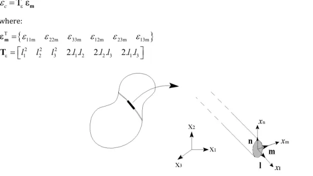
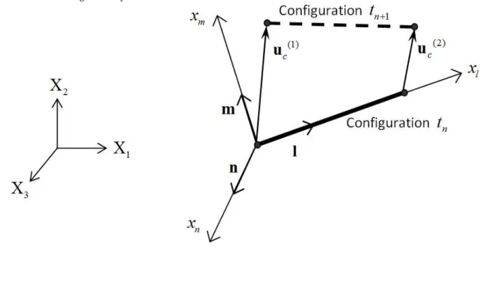
A basic assumption to be defined in embedded formulations is related to the strain field of the material in-volving a one-dimensional structure. Let us assume that the motion of any material point located on the contact surface between a curvilinear body, such as a bar or a cable, and the surrounding solid medium can be described using a local coordinate system attached to that curvilinear structure. In this system, the tangent direction is aligned with the longitudinal axis of the cable and the normal direction is related to any radial direction defined on the plane of its cross section (see Fig. 1). Depending on the physical problem, one can also assume that the contact along the normal direction is permanent and the normal component of relative displacement between the solid matrix and the cable is null, while the relative displacement in the tangential direction is not. This condition is called bond-slip and is valid when the surrounding material is sufficiently compact such that only tangential movements are permitted on the contact interface. A limit condition can be also adopted when no slip is allowed and the immersed curvilinear body adheres perfectly to the surrounding material. In the case of perfect adher-ence between reinforcement and the solid medium, the axial strain in the immersed cable εc can be obtained

(3)

c





 

_ _m ₍₁₎

where:



11m 22m 33m 12m 23m 13m



2 2 2

1 2 3

2. .

1 2

2. .

2 3

2. .

1 3

l

l l



 







 



m

T



(2)

Figure 1: Global and local coordinate systems.

Tensor εm is composed by strain components associated with the strain field of the surrounding material and

evaluated at the solid/cable interface. Notice that the curvilinear structural elements are modeled as flexible in-clusions (shear forces and bending moments are disregarded). Accordingly, compatibility condition (1) is simply expressing that the cable elements are endowed with the same kinematics as the embedding solid medium fol-lowing axial direction. The row matrix Tε is obtained from the second-order transformation matrix T usually

adopted during rotation of components of stress and strain tensors, which is given in the general case by:

2 2 2

1 2 3 1 2 2 3 1 3

2 2 2

1 2 3 1 2 2 3 1 3

2 2 2

1 2 3 1 2 2 3 1 3

1 1 2 2 3 3 1 2 2 1 2 3 3 2 3 1 1 3

1 1 2 2 3 3 1 2

2 .

.

l

l l

m

m m

n

n n

l m

l m l m

m n m n m n m n m n m n m n m n m n

l n

n l





T

2 1

.

2 3

.

3 2

.

3 1

.

1 3

.

n l

n l n l











































(3)

where li, mi and ni represent the direction cosines referring to the cable local axes (l, m, n) with respect to the

global coordinate system (X1, X2, X3).

When relative movement between the immersed cable and the surrounding material is considered, the dis-placement field in the solid matrix domain must be described using a composition of solid matrix disdis-placements and relative displacements at material points located on the solid/cable interface. In the present work, this com-position is only valid along the tangential direction of the immersed cable, whereas full bond between matrix and cable is assumed along the normal direction. Denoting by uc the cable displacement and by um that of the solid

matrix, the displacement jump along the matrix-cable interface may be expressed as:



c



m

s m c

u



u u



 

l

u u



(4)

with:









T









T

1 2 3

.

c,1 c,2 c,3

,

m 1 2 3

.

m,1 m,2 m,3

c

u



l l l

u



l l l

u

(5)

(4)

In infinitesimal framework, the weak form of the equilibrium condition applied to the mechanical system constituted by the solid matrix and embedded inclusions, takes the form:











int int



L

T T

L

d

dL

. d

d

dL

c c c s c

c c c c

u

P

u t

u

A

 







     

 

 

  

 

  

 





 





  

  



m c c

m m c c

m m m m c c

m m m m m m c c c

u t

u b

b





(6)

Subscripts m, c and int respectively refer to matrix, embedded cable and contact interface regions of the me-chanical system. Accordingly, Ωm and Γm define volume and boundary surfaces related to the spatial domain of the

matrix material, Ωc and Γc define volume and external surface related to the spatial domain of the cable, such that

Ωc = Ac.Lc and Γc = Pc.Lc, where Ac, Pc and Lc are the cross-section area, cross-section perimeter and length of the

immersed cable. The body forces acting on the system are denoted by vectors bm and bc, which generally reduce

to gravity. Stresses in the different components of mechanical system are denoted respectively by σm for matrix, σc for embedded inclusion and by τint for interface. The traction vector acting along Γm is denoted by

t

m, while

t

c

stands for the traction in axial direction of the embedded inclusion. In order to avoid volume superposition be-tween matrix and embedded cable when rigidity and geometrical characteristics are locally similar, integration of terms referring to the volume of the matrix material may be performed considering the following spatial domain:

m m c

d

_{    }



d

(7)

2.2 Constitutive equations for matrix and embedded inclusion

Relations between stress and strain are first presented to describe the constitutive equations of the matrix material considered in the present formulation. The state equation for the soil matrix phase is formulated within the framework of finite plasticity. Explicit rate-form expression involving the Jaumman derivative of the stress tensor as well as the associated corotational description is detailed in section 3.1. For the sake of clarity, the main features of the soil matrix constitutive behavior are provided in this section, restricting the description to the context of infinitesimal plasticity.

In the elastic range, the Cauchy stress tensor σm and the small strain tensor εm referring to the matrix

materi-al are related according to the following equation:

m



D

e

.

m





₍₈₎

where De_{is the fourth-order elastic constitutive tensor for an isotropic material, which may be described as:}

2

3

e

ijkl ik jl ij kl

D



G

  



_

K



G



_

 





(9)

where δij denotes the components of the Kroenecker delta and K and G are the bulk and shear moduli,

respectively. The incremental form of Eq. (8) is given as:





_m



D

e

.





_m.

In the elastoplastic range, the constitutive equation referring to the matrix material is described in the in-cremental form as follows:

ep

m m







D





(10)

with:

e T e g f ep e T e f g









D a a D

D

a D a

(11)

and: f g m m

;

m m

f

g







(5)

where κ is the hardening parameter,

f

m is the yield function and

g

m is the plastic potential. The total strain rate

is decomposed into elastic and plastic parts using the additive decomposition, that is:

e p

m m m



  

  



(13)

The flow rule is written as:

p m

m

g







 







(14)

where





is a positive scalar representing the plastic multiplier. The complete description of the elastoplastic formulation requires the yield function

f

m, the plastic potential

g

m and a hardening law to be prescribed. In the

present work, the generalized formulation presented in references (Nayak and Zienkiewicz 1972; Owen and Hinton, 1980; Souza Neto et al., 2008) is adopted to describe the material models utilized here for the matrix material.

As regards the embedded inclusions, an elastic behavior is considered in the analysis, with account for geo-metric nonlinearities. The specific state equation for inclusions will be described in section 3.2. Meanwhile, it takes the following form in the context of infinitesimal elasticity:

c

Ε

c c







₍₁₅₎

where σc and εc are the axial components of the Cauchy stress and small strain tensors, respectively, and Ec is the

Young modulus of the constitutive material. The incremental form of Eq. (15) may be expressed as

 



c

Ε

c





c .

2.3 Constitutive behavior for interface material

We address hereafter the elastoplastic constitutive formulation referring to the contact interface. The differ-ential form of the total relative displacement on the interface is decomposed into reversible and irreversible parts, which are described according to the local coordinate system defined in terms of tangential and normal components, that is:

el ir

s s s

du



du



du

(16)

el ir

n n n

du



du



du

 

(17)

where superscripts el and ir indicate the reversible and irreversible parts of the corresponding jump displacement components. Notice that the total relative displacement in the normal direction is zero owing to the assumption of bond-slip contact at the interface.

(6)

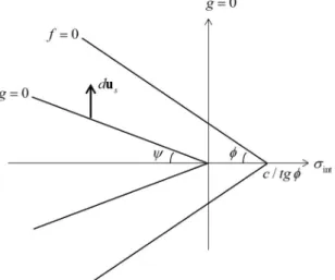
In order to define the interval of stress states that correspond to reversible relative displacements, a yield criterion must be defined. In the present work, the Mohr-Coulomb yield criterion is adopted (see Fig. 2):

int int

f











c

(18)

where c is the cohesion and μ is the friction coefficient of the material interface. Coefficient μ is usually defined from the internal friction angle ϕ:





tg



. The stress vector acting upon a current point of the interface is defined in terms of the tangential (τint) and normal (σint) stress components. The tangential stress component is

updated according to the elastic-plastic formulation, where the yield criterion described above indicates if the stress increment associated with the relative displacement on the interface is obtained using an elastic constitutive equation or an elastic-plastic constitutive equation.

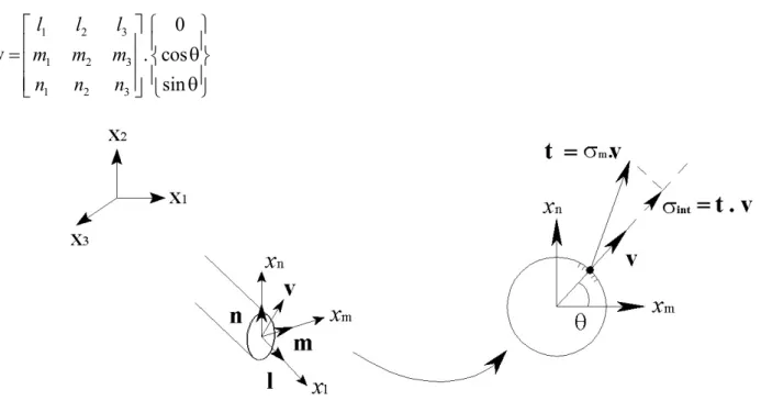
We deal now with the crucial issue related to how the normal vector v to cylindrical interface can be defined in the plane of inclusion cross-section (see Fig. 3). It is emphasized that this key point is inherent to the mixed 3D-1D formulation when the interface behavior is accounted for. The underlying question is: how interaction forces between a 1D structural element and the surrounding 3D continuous body are possibly modeled from a rigorous mechanical viewpoint? An approximate approach to deal with this challenging issue has been proposed in Figueiredo et al. (2013). In the subsequent analysis, we develop a heuristic approach in which interaction efforts are defined from minimization of the shear component of the stress vector generated on all the facets of the soil/inclusion interface by the stress tensor in the soil. The stress vector acting along the interface is first comput-ed from the stress tensor σm in the solid matrix:

m





t



v

(19)

The normal stress is simply the projection of

t

on the normal direction:

int



 

_{t v}

₍₂₀₎

From a computational viewpoint, tensor σm is evaluated at macroscopic points of the matrix element

contain-ing the inclusion element, coincidcontain-ing with the integration points of the inclusion element. Unit normal vector v is defined in the global coordinate system (X1, X2, X3) by its orientation θ in the inclusion cross-section plane and the

direction cosines li, mi and ni of the local frame (l, m, n):

1 2 3

cos

sin

l

m m m

n





 











_

_



_



_











 



v

(21)

Figure 3: Stress vector acting at matrix/inclusion interface and corresponding normal component.

(7)

considers the orientation



that minimizes the value of shear stress

c





int complying with the yield criterion (18). This arbitrary definition implicitly assumes a constant stress state when moving around the soil/inclusion interface, which could reveal questionable in some situations. It is readily shown that condition dσint/dθ = 0

yields:

tg2

C



 

 

(22)

with:

2 2 2

m 2

l

m 2

m

m 2

n

2

m 2 2

l m

2

m 2 2

l n

2

m 2 2

m n



_



_



_



_



_



_

 



₍₂₃₎













m 2 3 m 2 3 m 2 3

m 2 3 3 2 m 2 3 3 2 m 2 3 3 2

B 2

2

2 l l

m m

n n

l m l m

l n l n

m n m n



  

  





(24)

2 2 2

m 3 m 3 m 3 m 3 3 m 3 3 m 3 3

C





_

l





_

m





_

n



2 

_

l m



2 

_

l n



2 

_

m n

(25)

The solution to Equation (22) that leads to higher value of



int is hence retained.

The direction of relative plastic displacement is derived from the flow rule given as follows:

int

ir

s

g

du

d













(26) int ir n

g

du

d













(27)

where

d





is the plastic multiplier and g is the plastic potential. The latter is assumed under form:

int int

g







tg

 

(28)

where

 



is the dilatancy angle.

The consistency condition employed in the present formulation may be expressed as:

int int

f

_{f c 0}

c

d



d



d













(29)

The last term of the equation above is related to material hardening when this feature is considered in the mechanical description of the material. A linear isotropic strain hardening model is assumed here to describe the cohesion evolution after yielding, which may be expressed as follows:

c

ir

s

d



h du

(30)

where h is the hardening modulus. Notice that the cohesion evolution does not explicitly depend on the normal component of the stress state along the interface.

Recalling that the normal component of the total relative displacement

du

n is zero, one obtains:

int

0

el ir el

n n n

g

du

d















 



(31)

The elastic constitutive equation describing the behavior of interface written in terms of differential stress components and differential relative displacements reads:

int int el n n el s s

d

k du

d

k du

(8)

in which kn and ks refer to normal and tangential stiffness moduli. It is observed that these quantities are

expressed in units of force per cubic length [Pa/m].

By substituting Eq. (31) into the constitutive equation corresponding to the normal stress component, the plastic multiplier can be obtained as follows:

int

tg

n

d

k







  

(33)

On the other hand, making use of the consistency equation together with constitutive equations (32) leads to:

int int

( )

h d

´

d

sign

tg















(34)

Finally, the plastic multiplier may be rewritten as follows:

int int int

( )

n

sign

d

k tg tg

h sign







 



 



(35)

It stems from the constitutive equation of the interface following the tangential direction that:





int

ir

s s s s s

g

d



k du du

k du d







_











_



_







(36)

Taking into account the particular form (28) of potential

g

and expression (35) of plastic multiplier, the elastoplastic constitutive equation of the matrix-reinforcement interface is given as follows:

int int

1 ( )

s s s n

k

d

_k

du

k tg tg

h sign



 







(37)

Therefore, the incremental form of the constitutive equations referring to the contact interface reads:

int

k u

s s





 

₍₃₈₎

in the elastic range, and:

int int

1 ( )

s s s n

k

_u

k

k tg tg

h sign



 











(39)

in the plastic range. When





0

(no dilation), condition

du

n



0

can be ensured by choosing

k k

n

/ ~1/

s

tg



.

3 FINITE STRAIN APPROACH

Nonlinear problems are usually analyzed employing the incremental approach, where strain increments are evaluated based on the last incremental displacement field obtained from the solution of the equilibrium equa-tions. At each iterative step, the respective stress updates are obtained according to the material behavior. When large strains are involved, the latter can be described in the corotational coordinate system adopting objective stress rate.

Although the matrix and the inclusions may undergo large strains, a fundamental assumption of the present modeling is that the strains along matrix/inclusions interface remain infinitesimal.

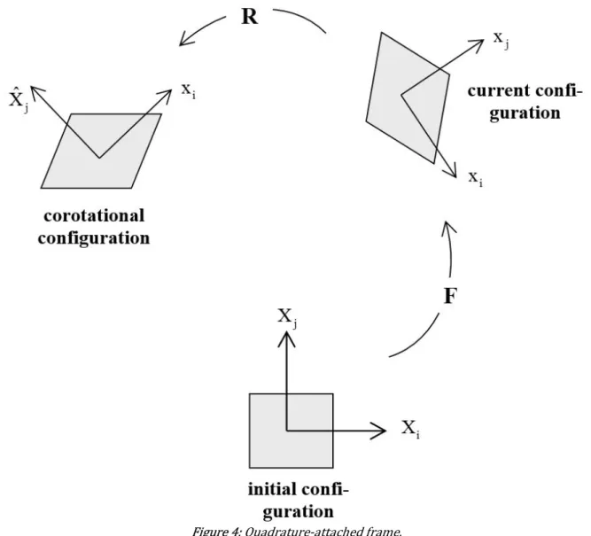
3.1 Corotational description of matrix particles motion

(9)

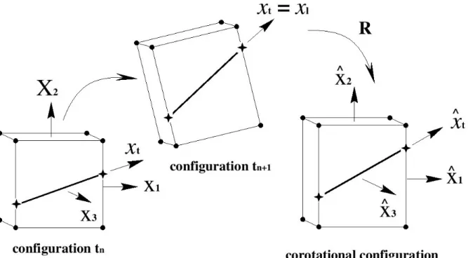
configura-tion usually refers to the undeformed configuraconfigura-tion, while the corotated one is obtained through a rigid body tion from the base configuration. The coordinate system of the corotated configuration follows the material mo-tion and can be easily related to the global coordinate system through rotamo-tion operamo-tions. In the finite element approach, each element possesses its own set of coordinate systems located at the respective quadrature points.

Figure 4: Quadrature-attached frame.

The starting point of the analysis is the decomposition of geometric transformation of matrix into a rigid body motion and pure deformation performed at the element level in the corotational coordinate system. Such a corotational description maintains orthogonality of the attached reference frame as illustrated in Figure 4, thus providing an effective setting for rate form formulation of the constitutive equations in the context of large strains. Note that rotation

R

transforming the current configuration into corotational configuration can be de-fined from the rotation component in polar decomposition of deformation gradient (Espath et al., 2014).

Assuming that all kinematical variables are known at the previous configuration t = tn of the matrix, the

dis-placement field at the end of the current load step can be obtained from integration of the strain rate tensor along time interval [tn, tn+1]. The whole steps of the reasoning are performed in the corotational coordinate system,

where notation



ˆ

shall be used to express any field



in the corotational frame. The strain rate tensor in the corotational system is defined as:

T def def

m m

m

ˆ

1 ˆ

ˆ

2 

_

_

_

_





_{ }

_

















v

d

x

(10)

where

v

ˆ

defm represents the velocity field associated with the deformation part of the motion expressed in the

corotational system. The strain increment is computed using the mid-point integration proposed in Hughes and Winget (1980). In this procedure the velocity is assumed to be constant within the time interval and the reference configuration is attached to the intermediate configuration at t = tn+1/2 in the corotational system. Accordingly:

1 def def T

m m

n 1 2 n 1 2

ˆ

1 ˆ

_d

_ˆ

ˆ

2

n n t t



  



_

_

_

_













_



_

 





_

_









d

u

x



(41)

where



u

ˆ

defm is referred to the deformation part of the total displacement increment



u

ˆ

m in the corotational system and

x

ˆ

n 1 2 is the intermediate geometric configuration of the matrix element in the corotational system,

which can be computed as:





n+1 2 n+1 2 n+1 2

1

n+1 2 n n+1

ˆ

2 









x

R

x

R

x x

(42)

where

R

n+1 2 is the orthogonal transformation tensor performing rotation from the global coordinate system to

the corotational coordinate system defined locally at the intermediate configuration

t

n1/2 of the matrix element. The displacement increment



u

m referring to time interval [tn, tn+1] is decomposed at element level according to:

def rot

m m m



u

 

u

 

u

(43)

In the above local relationship,



u

def_m and



u

rot_m denote respectively the deformation and rotation parts of the displacement increment defined in the global coordinate system.

The increment of deformation displacements expressed in the corotational system is defined by:

def def

m n 1 n n+1 2 m

ˆ

_

ˆ



u



x



x



R

 

u

(44)

since the strain rate tensor is evaluated at the intermediate configuration

t

n1/2. Coordinates

x

ˆ

n and

x

ˆ

n 1 corresponding to geometric configurations in the corotational system at

t t



n and

t t



n1 are obtained from the following transformations:

n n n n+1 n+1 n+1

ˆ





and

ˆ





x R x

x

R

x

(45)

where

R

n and

R

n+1are orthogonal transformation tensors performing rotations from the global coordinate system to the corotational coordinate system defined locally at

t t



n and

t t



n1, respectively. Vectors

x

n and

n+1

x

refer to geometric configurations defined in the global coordinate system. Omitting subscripts



n n

,



1/ 2,

n



1 

referring to considered time, the components of the transformation

R

are given by:

1j 2j cj 3j

1j T 2j T 3j T

1 1 2j cj 2j cj 3 3

)

;

(j 1,2,3)

)







r

(r

r

R

r r

(r

r (r r

r r

(46)

with:

T 1j 2j

T T

1j j 2j j cj T 1j 3j 1j 2j cj

1j 1j

;

(

)



 

r r

 



r

x

r

x

r

r r





(47)

(11)

The Cauchy stress tensor in the global system is obtained from objective tensor transformation as follows:

T m



R

ˆ

m

R



₍₄₈₎

where



m and



ˆ

m are the Cauchy stress tensors evaluated in the global and corotational system, respectively. To formulate the constitutive behavior of matrix constitutive material, a set of assumptions are stated. First, the elastic part of the deformation gradient of matrix particles is assumed to remain infinitesimal, meaning that large strains are of irreversible (plastic) nature. In addition, the constitutive material is considered as elastically isotropic and that elastic properties are not affected by the plastic strains. Under these conditions, it can be shown that the state equation formulated in rate form relates a rotational time derivative of stress tensor (Jaumman derivative) and the strain rate tensor (see for instance Dormieux and Maghous, 1999; Bernaud et al., 2002; Bernaud et al., 2006) through:





J e p J

m

ˆ

m

ˆ

m m m m

ˆ

m

ˆ

m m

ˆ

D d



d

with

ˆ

+

ˆ

    

ˆ



 

  

  



(49)

where

d

ˆ

pm denotes the plastic strain rate and



ˆ

mis the spin tensor defined in the corotational system. The above

equation is used for stress updates in the corotational system in the context of large strains. It is observed that the corotational spin tensor has also to be integrated over the time interval

[ ,

t t

n n1

]

following the same mid-point rule adopted in (41).

3.2 Description of deformation in embedded inclusion

As adopted for surrounding matrix, the kinematics of the embedded inclusion is described referring to con-figuration

t

n. With respect to this configuration, the Green-Lagrange axial strain writes:

c c

1 ₂

with

c c

t t t

u

_u

x





 









_

_{ }

_







_



c

_{ }



c

_

u

_{u l}

E

(50)

where

u

c is the displacement vector at any point along the embedded inclusion. Derivations are taken with respect to coordinate

x x

t



l along the tangential direction, as illustrated in Figure 5.

It is recalled that the displacement jump at the surrounding matrix/inclusion interface is purely tangential (see section 2.1):

c



m



u

s

u u

l

(51)

where

l

is the unit vector along the cable. Accordingly, the components of

u

c in the local coordinate system may be expressed from

u

sand the displacement components in the global coordinate system umT = (um,1, um,2, um,3) of

the geometrically coinciding matrix particle:

1 2 3 m,1

1 2 3 m,2

1 2 3 m,3

0

s

u

l

u

m m

m

u

n

u







  



 













_{ }



_

_



_

_

 

_

_



  

 



c m

(12)

Figure 5: Displacements of an element of embedded inclusion.

As defined in Figure 1, li, mi and ni are the direction cosines of inclusion local axes

(

l , m ,n

)

with respect to

the global coordinate system

( ,

X X X

1 2

, )

3 . Matrix

R

 is the coordinate rotation transformation between local and global frames.

The axial strain

E

c is computed using the matrix notation (52):

1

2

3

0

c t s t m m m

c t m m m

t

c t m m m

u x

u

x

u

y

u

z l

v x

v

x

v

y

v

z l

x

w x

w

x

w

y

w

z l







 





  



_{ }



_

_

 

_{ }

_



_

_{ }



_



 

_{ }







_

_{ }

_

_{ }









 





  

c

u

_{+ R}

(53)

The embedded curvilinear inclusion is discretized by means of succession of linear elements. Each element is embedded within a brick element (parent element) associated with a constant tangent vector

l

and a constant matrix transfer R*. When perfect bonding is considered at the interface solid matrix/inclusion, the first term in the right hand-side of (53) should be removed (i.e.,

  

u x

s t

0

).

(13)

Figure 6: Updated Lagrangian scheme and corotational configuration in the context of embedded approach.

Assuming an elastic behavior for the inclusion constitutive material, the stress increment during time inter-val

[ ,

t t

n n1

]

is related to axial strain by means of the uniaxial linear relationship:

c

E



 

E

(54)



is the second Piola-Kirchhoff stress tensor and

E

c is the elastic stiffness of the inclusion constitutive material. 3.3 Finite element discretization

In the subsequent analysis the eight-node hexahedral finite element formulation with one-point quadrature is adopted to discretize the displacements of matrix particles. At the element level, the displacement vector of matrix particles between

t

n and

t

n1 is approximated, using Voigt notation, as follows:

1

m

with

m

n n

t t 















_{ }

_









m m m m

N 0 0

u

x

N u

N

0 N 0

0 0 N

(55)

where

u

m is the vector of nodal displacements referring to eight-node hexahedral element and

N

mis the 3 24 matrix defined by sub-matrix

N





N ,

1



, N

8



that contains the associated shape functions. In the context of

geometrically nonlinear analysis, these quantities are evaluated considering the current configuration of the element in the corotational coordinate system (

u

ˆ

_mand

N

ˆ

m, respectively). At element level, the strain increment

is thus computed according to:



(14)

m

B

being the 3 24 _{matrix aimed to generate the symmetric part of the displacement gradient at element} level (see Eq. (41)). It is should be observed that matrix

B

m must be also evaluated considering the differential

operator in the corotational coordinate system, that is operating with

B

ˆ

m. Finally, similar procedures are used

for the finite element approximation of strain rate tensor and spin tensor.

Regarding the embedded inclusions, their geometry is discretized into piecewise linear elements. Instead of nodal displacements of the inclusion elements, the approach operates with nodal displacements jump. Along each two-node element, the tangential relative displacement between matrix and inclusion particles defined in (4) is approximated from the nodal values:

s

u

_



s

u



₍₅₇₎

where

u

s is the tangential displacement jump vector related to the linear finite element nodes of the embedded inclusion. Matrix Φ, whose dimension is 1 2 , contains the shape functions of the two-node linear element.

Recalling that

u

c



u

s

l +R u





m (see equations (51) and (52)), the discretized expression of axial Green-Lagrange strain between

t

n and

t

n1 reads in each inclusion element:

T T c





s

u

s



 

 m

u

m



₂

1 d G G d

 

E

(58) where t

d

dx



s

B



is the 1 2 matrix containing the derivatives of shape functions with respect to tangential

coordinate along the inclusion element,

T

is the 1 6 matrix introduced in (2). Matrix

G

, whose dimensions are

3 26 , is defined by:

1 j 2 j 3 j

j j j t

1 j 2 j 3 j

j j j

1 j 2 j 3 j

j j j

l l

x

m l

x

n l

x



_





_









_

















_

















N

G

0 N

N

₀



(59)

Vector

d

contains 26 components of nodal displacements associated with the matrix element (brick ele-ment) and embedded linear inclusion element:

  













m s

u

d =

u

(60)

Rearranging (58) yields:





T T

c



 

 m



s

d





1 ₂

d G G d

 

E

(61)

It is observed that



 

 m



s



is a 1 26 matrix defined from sub-matrices

 

 m and



s. If perfect bonding is considered at the matrix/inclusion interface, the latter expression reduces to

T T c



 

 m

u

m



₂

1 u G G u

m

 

m

E

(62)

(15)

The subsequent developments deal with the finite element formulation of the equations governing the re-sponse of the mechanical system to a prescribed external loading. It is recalled that the mechanical system refers to the solid matrix and embedded inclusions in mutual interaction. Discretization of the weak form of balance momentum expressed at current configuration of the mechanical system results in a set of nonlinear equations. These equilibrium equations must be iteratively satisfied using the incremental approach (see Bathe, 1996), since both the stiffness matrices and the internal force vectors are functions of the current element configuration. A linearization procedure based on Newton-Raphson method and Taylor series expansion of the general internal force vector within the time interval

[ ,

t t

n n1

]

leads to the following global system:

tan ext int

n 1,i 1 

( )

n+1,i



n 1



n 1,i 1 

( )

K

U U

F

U

(63)

where subscript

n



1

denotes the current position in the time marching, while subscripts

i

and

i



1

refer respectively to current and previous iterative steps in the Newton-Raphson procedure applied over the time interval

[ ,

t t

n n1

]

.

K

tan is the tangent stiffness matrix,

F

ext and

F

int are the external and internal force vectors, respectively.

U

represents the global vector whose components are node values of the matrix displacement and the interface relative displacement between

t

_n and

t

n1. Vector

U

is obtained by assembling procedure to incorporate the contribution of all element nodal displacements

u

m or

d

.

At each iterative step, the stiffness matrix and the internal force vector are evaluated in the corotational co-ordinate system. In particular, the terms related to the elementary contribution of matrix (matrix element with-out embedded inclusion) take the following expressions:





T ep geo int T

m

ˆ ˆ

ˆ

_d

ˆ

_;

ˆ

_ˆ

_d

ˆ

e e

m m

e e

m m

 



_







_



tan

m m m m m

k

B D

D

B

f

B



(64)

where



ˆ

em stands for the current configuration of the matrix element volume in the corotational system.

D

ˆ

ep is

the stress-strain constitutive matrix defined in (49),

D

ˆ

geo is the geometric stiffness matrix associated with the Jaumann rate terms



ˆ

m

    

ˆ

m

ˆ

m



ˆ

m, and



ˆ

m is the corotational Cauchy stress tensor (see Braun and Awruch, 2008; Duarte Filho and Awruch, 2004 for further details). In order to solve the equilibrium equation, the tangent stiffness matrix and the internal force vector are brought back to the global coordinate system using the following objective transformations:

tan

_

T

ˆ

tan

_;

int

_

T int

ˆ

m m m m

k

R k R

f

R f

(65)

where

R

is the rotation transformation matrix defined in Eqs. (45) and (46).

The finite element formulation is based on reduced integration, where hourglass control techniques are employed in order to avoid numerical instabilities, such as volumetric locking and/or shear locking. Detailed description of the stabilization procedures adopted in this work may be found in Braun and Awruch (2008, 2013).

As regards the contribution of embedded inclusions to tangent stiffness matrix and force vector, the work performed by the internal axial force  in any virtual elastic evolution



E

c should be analyzed. Denoting by



ˆ

ec

the last equilibrated configuration of the inclusion element with respect to the corotational system of the sur-rounding matrix element (parent element), the internal force vector related to inclusion element is defined as:

T

int T

s

ˆ ˆ

ˆ

_d

ˆ

ˆ ˆ

_d

ˆ

e e

c c

e e

c c









 









_

_

 





c m

f

 



G G d

(66)

(16)

T _T

s c s

ˆ ˆ

ˆ

_E

ˆ

_d

ˆ

_d

ˆ

e e

c c

e e

c



c c

 

 













_

_

_

_

 





tan

c m m

k

 



 



G G

(67)

where

E

cis the longitudinal elastic stiffness of inclusion material and



c is the axial Cauchy stress tensor along

the inclusion element.

For a single element with embedded inclusion segment, the discretized weak form of equilibrium equation writes

 

n 1,i n 1

n 1,i 1 n 1,i 1

       













_







_







_











_















_

























int int ext ext

mm mm,cc mc m m m,c m m,c

G ext int int

cm cc ss s s s s,c

k

_k

u

f

k

u

f

(68)

where:





T ep geo ˆ

ˆ

_with

ˆ

_d

ˆ

e m





T



_





mm mm mm m m

k

R k

R

k

B D

D

B

(69)

T c c ˆL

ˆ

_with

ˆ

_{E A}

ˆ

_dL

ˆ

e c e c  











T

_{ }

_

_

_

_

mm,cc mm,cc mm,cc m m

k

R k

R

k

 

(70)

T

s c c s ˆL

ˆ

_with

ˆ

_{E A}

ˆ

_dL

ˆ

e c



T





cc cc cc

k

R k R

k



(71)

T

c c s ˆL

ˆ

_with

ˆ

_{E A}

ˆ

_dL

ˆ

e c e c 







T

_{ }



_

mc mc mc m

k

R k R

k

 



(72)

T s c c ˆL

ˆ

_with

ˆ

_{E A}

ˆ

_dL

ˆ

e c e c 







T





_

_

cm cm cm m

k

R k R

k



 

(73)

b,t c ˆL

ˆ

_with

ˆ

_K

_{P dL}

ˆ

e c



T





ss ss ss

k

R k R

k

_



_

₍₇₄₎

T

ˆ

ˆ ˆ

_d

ˆ

e c e c c











G

k

G G

(75)

T

ˆ

_with

ˆ

_ˆ

_d

ˆ

e m e m 



_



int T int int

m m m m m

f

R f

f

B



(76)

T c ˆL

ˆ

_with

ˆ

_{A dL}

ˆ

e c e c c











_{ }



_

int T int int

m,c m,c m,c m

f

R f

f

 

(77)

int c ˆL

ˆ

_with

ˆ

_{P dL}

ˆ

e c e c







int T int int

s s s

f

R f

f

_

 ₍₇₈₎

T

s c

ˆL

ˆ

_with

ˆ

_{A dL}

ˆ

e c e c c





_

int T int int

s,c s,c s,c

f

R f

f



(79)

T T m m ˆ ˆ

ˆ

d

e e

m m m

e

m m

   



_

 

_



ext

m m m

f

N t

N b

(80)

T T

m m c

ˆ _ˆL

ˆ

d

A dL

e e

c c c

e

c c

  



_

 

_

ext

m,c c c

(17)









T T

c

ˆ _ˆL

ˆ

d

A dL

e e

c c cc

e

c c

  



_



 

_



ext

s c c

f



t l



b l

(82)

For a matrix element without embedded inclusion, (68) reduces to:





n 1,i 1_{ }

 

_ n 1,i

   

n 1 n 1,i 1 



ext



int

mm m m m

k

u

f

(83)

After assembling all the elements, the global system takes the form given by Eq. (63), which is solved itera-tively with implementation of Generalized Displacement Control Method (e.g. Yang and Shieh, 1990).

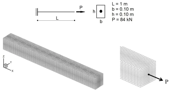
4 VERIFICATION TEST OF NUMERICAL PROCEDURE

In order to check the finite element implementation of the proposed model as well as related accuracy, the numerical simulation of a kind of inclusion pull-out test is analyzed in the sequel. The structure sketched in Fig. 7 consists of a reinforced cantilever beam with length L and rectangular b x h cross-section. The loading is defined by the following conditions:

• body forces are neglected;

• both matrix and inclusion are clamped along the plane x = 0;

• a force

Pe

_x is applied at the free end of the reinforcing inclusion, while the matrix is free of stresses along the plane x = L.

The matrix constituent material is elastic perfectly plastic with a von Mises condition for plastic yielding. A Mohr-Coulomb elastoplastic constitutive law with a non associated plastic flow is considered for the ma-trix/inclusion interface. The corresponding model data are given in Table 1. The finite element grid used for the simulation is shown in Fig. 7 and consisted of 110x20x20 hexahedral eight-node elements, resulting from a pre-liminary mesh sensitivity (convergence) analysis. The influence of interface properties on the structure response is investigated by varying the value of two typical parameters, namely the interface elastic stiffness

k

s and the

interface cohesion c.

(18)

Table 1: Material properties for the inclusion pull-out test.

Properties Values

Matrix

Elastic modulus

E

25000 MPa

Poisson ratio 

_0.2

Yield strength



y

2.2 MPa

Inclusion Cross-section area

A

c

4 2

1.0 10 m

_



Elastic modulus

E

_c

210000 MPa

Soil-cable interface

Tangential stiffness modulus

k

_s

2.0 10 2.0 10 Pa / m



1





11

Normal stiffness modulus

k

_n

10

6



k

_s

Cohesion c

0.25 1.0 kPa



Internal friction angle



₃₀



Dilatancy angle



₀



Table 2 summarizes the numerical predictions derived from the formulation implemented in this paper, to-gether with the finite element solutions obtained from ANSYS software. The latter has been used considering hex-ahedral 20-node elements (SOLID 95) for both the matrix and inclusion domains, while quadrilateral 8-node ele-ments (CONTA 174 and TARGE 170) have been used for the contact interface. The structural response is evaluat-ed by computing the axial displacement

u

cmax



u x L

c

(



)

at the free end of the inclusion (loaded point), the

rela-tive tangential displacement

u

maxs



u x L

s

(



)

at the same point, and the reaction force

R

applied to the

inclu-sion at its fixed (clamped) end (

x



0

). As it can be observed from this comparison, a good agreement is obtained from the two distinct numerical approaches, thus providing a first validation of the proposed numerical formula-tion. The accuracy of the latter can be illustrated by evaluating the maximum relative difference observed be-tween the two approaches considering the 36 simulations that are reported in Table 2: displacement at inclusion free end



u

cmax

/

u

cmax



3.5%

; relative displacement at inclusion fixed end



u

smax

/

u

smax



11.5%

; reaction

(19)

Table 2: Results obtained from numerical simulations of the inclusion pull-out test.

c (MPa) Ks

(Pa/m)

max

s

u

(m)

max

s

u – ANSYS

(m)

max c

u

(m)

max c

u – ANSYS

(m)

R

(KN) R – ANSYS (KN)

0.25

2.0x101 _4.00x10-3 _4.00x10-3 _4.00x10-3 _4.00x10-3 ₈₄ ₈₄

2.0x103 _4.00x10-3 _4.00x10-3 _4.00x10-3 _4.00x10-3 ₈₄ ₈₄

2.0x105 _4.00x10-3 _4.00x10-3 _4.00x10-3 _4.00x10-3 ₈₄ ₈₄

2.0x106 _3.99x10-3 _4.00x10-3 _4.00x10-3 _4.00x10-3 _83.9 _83.9

2.0x107 _3.95x10-3 _3.96x10-3 _3.95x10-3 _3.96x10-3 _82.5 _82.7

2.0x108 _3.78x10-3 _3.80x10-3 _3.80x10-3 _3.82x10-3 _76.6 _77.1

2.0x109 _3.77x10-3 _3.79x10-3 _3.78x10-3 _3.81x10-3 _75.1 _76.1

2.0x1010_3.71x10-3 _3.79x10-3 _3.73x10-3 _3.81x10-3 _73.4 ₇₆

2.0x1011_3.71x10-3 _3.79x10-3 _3.73x10-3 _3.81x10-3 _73.4 ₇₆

0.5

2.0x101 _4.00x10-3 _4.00x10-3 _4.00x10-3 _4.00x10-3 ₈₄ ₈₄

2.0x103 _4.00x10-3 _4.00x10-3 _4.00x10-3 _4.00x10-3 ₈₄ ₈₄

2.0x105 _4.00x10-3 _4.00x10-3 _4.00x10-3 _4.00x10-3 ₈₄ ₈₄

2.0x106 _3.99x10-3 _4.00x10-3 _4.00x10-3 _4.00x10-3 _83.9 _83.9

2.0x107 _3.95x10-3 _3.96x10-3 _3.95x10-3 _3.96x10-3 _82.5 _82.7

2.0x108 _3.62x10-3 _3.66x10-3 _3.65x10-3 _3.68x10-3 _72.4 _73.3

2.0x109 _3.54x10-3 _3.59x10-3 _3.57x10-3 _3.62x10-3 _66.8 _68.3

2.0x1010_3.48x10-3 _3.59x10-3 _3.52x10-3 _3.62x10-3 _64.6 ₆₈

2.0x1011_3.45x10-3 _3.59x10-3 _3.49x10-3 _3.62x10-3 _63.6 ₆₈

0.75

2.0x101 _4.00x10-3 _4.00x10-3 _4.00x10-3 _4.00x10-3 ₈₄ ₈₄

2.0x103 _4.00x10-3 _4.00x10-3 _4.00x10-3 _4.00x10-3 ₈₄ ₈₄

2.0x105 _4.00x10-3 _4.00x10-3 _4.00x10-3 _4.00x10-3 ₈₄ ₈₄

2.0x106 _3.99x10-3 _4.00x10-3 _4.00x10-3 _4.00x10-3 _83.9 _83.9

2.0x107 _3.95x10-3 _3.96x10-3 _3.95x10-3 _3.96x10-3 _82.5 _82.7

2.0x108 _3.56x10-3 _3.61x10-3 _3.59x10-3 _3.64x10-3 _71.2 _72.3

2.0x109 _3.03x10-3 _3.24x10-3 _3.39x10-3 _3.44x10-3 _61.4 _61.3

2.0x1010_2.73x10-3 _2.99x10-3 _3.37x10-3 _3.44x10-3 _60.7 ₆₀

2.0x1011_2.64x10-3 _2.99x10-3 _3.35x10-3 _3.44x10-3 _59.6 _59.7

1.0

2.0x101 _4.00x10-3 _4.00x10-3 _4.00x10-3 _4.00x10-3 ₈₄ ₈₄

2.0x103 _4.00x10-3 _4.00x10-3 _4.00x10-3 _4.00x10-3 ₈₄ ₈₄

2.0x105 _4.00x10-3 _4.00x10-3 _4.00x10-3 _4.00x10-3 ₈₄ ₈₄

2.0x106 _3.99x10-3 _4.00x10-3 _4.00x10-3 _4.00x10-3 _83.9 _83.9

2.0x107 _3.95x10-3 _3.96x10-3 _3.95x10-3 _3.96x10-3 _82.5 _82.7

2.0x108 _3.56x10-3 _3.61x10-3 _3.59x10-3 _3.64x10-3 _71.2 _72.3

2.0x109 _2.39x10-3 _2.55x10-3 _3.28x10-3 _3.33x10-3 _61.4 _61.4

2.0x1010_2.09x10-3 _2.34x10-3 _3.27x10-3 _3.33x10-3 _60.5 _59.9

2.0x1011_2.04x10-3 _2.31x10-3 _3.27x10-3 _3.33x10-3 _60.3 _59.2

Figure 8 shows the relative displacements at the matrix/inclusion interface along the beam longitudinal axis.

The curves

u u x

s



s

( )

are displayed for each value of the interface cohesion



0.25 MPa, 0.5 MPa, 0.75 MPa, 1.0 MPa



c _{, the tangential elastic stiffness being kept constant equal to}

9

2.0 10 Pa / m

s

(20)

Figure 8: Numerical predictions of relative displacement profiles along the matrix/inclusion interface

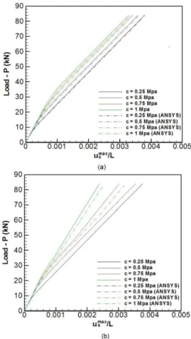
Figures 9a and 9b display the load-strain curves characterizing the response of the reinforced beam under pull-out test. Fixing the value of interface tangential elastic stiffness to

k

s



2.0 10 Pa / m



9 , the plots of

ap-plied force

P

versus normalized axial displacement

u

cmax

/

L

(Fig. 9a) and versus normalized tangential relative

displacement

u

smax

/

L

(Fig. 9b) at the free end are shown for the different values of interface cohesion.

Compari-sons of the numerical model with the analysis using ANSYS corroborate the previous comments referring to the validity of the numerical procedure.

Figure 9: Load-strain curves for the inclusion pull-out test: (a) applied force versus

u

cmax

/

L

; (b) applied force versus

max

_/

s