Lat. Am. j. solids struct. vol.13 número8

Abstract

Modeling and simulation of mechanical response of structures, relies on the use of computational models. Therefore, verification and validation procedures are the primary means of assessing accuracy, confidence and credibility in modeling. This paper is concerned with the validation of a three dimensional numerical model based on the finite element method suitable for the dynam-ic analysis of soil-structure interaction problems. The soil mass, structure, structure’s foundation and the appropriate boundary conditions can be represented altogether in a single model by using a direct approach. The theory of porous media of Biot is used to represent the soil mass as a two-phase material which is considered to be fully saturated with water; meanwhile other parts of the system are treated as one-phase materials. Plasticity of the soil mass is the main source of non-linearity in the problem and therefore an iterative-incremental algorithm based on the Newton-Raphson procedure is used to solve the nonlinear equilibrium equations. For discretization in time, the Generalized Newmark-β method is used. The soil is represented by a plasticity-based, effec-tive-stress constitutive model suitable for liquefaction. Validation of the present numerical model is done by comparing analytical and centrifuge test results of soil and soil-pile systems with those results obtained with the present numerical model. A soil-pile-structure interaction problem is also presented in order to shown the potentiality of the numerical tool.

Keywords

Soil-structure interaction, fully coupled analysis, porous media, finite elements

On the Validation of a Numerical Model for the Analysis

of Soil-Structure Interaction Problems

Jorge Luis Palomino Tamayo a Armando Miguel Awruch b

a _{Center of Applied Mechanics and}

Com-putational (CEMACOM), Engineering School of Federal University of Rio Grande do Sul, Av. Osvaldo Aranha 99-3o Floor, 90035-190, Porto Alegre, RS, Brazil, lpt.jorge@gmail.com

b _{Department of Civil Engineering,}

Engi-neering School Federal University of Rio Grande do Sul, Av. Osvaldo Aranha 99-3o _{Floor, 90035-190, Porto Alegre, RS,} Brazil, +55(51)-33083450,

amawruch@ufrgs.br

http://dx.doi.org/10.1590/1679-78252450

1 INTRODUCTION

The soil-structure interaction in general has been a concern and there is a need to further under-stand and better model this interaction. Civil structures are commonly supported on reinforced concrete shallow or deep foundations. When the rock basement of the soil deposit is far from the soil surface and the shear resistance of the soil is adequate, deep foundations made of concrete piles are typically used. In this way, proper numerical analyses of these structures are of importance for the civil and geotechnical engineering community in order to improve designs in terms of safety and economy. The main function of piles is to transferred axial an lateral loads from the superstructure to a reliable soil. Thus, several studies have been advocated to the study of soil-pile interaction problems under lateral and axial loads by using simplifying or complex approaches (Taiebat and Carter, 2001, Gu et al., 2016,Khoadir and Mohti, 2014, Chatterjee et al., 2015). Other research groups have focused on the development of simplified expressions for evaluating pile displacements and bending moments along the pile axis (Khodair and Mohti, 2014) by using the subgrade reaction approach (Valsamis 2008, Valsamis et al. 2012, Chaloulos et al. 2013b). In this approach, the pile is treated as an elastic laterally loaded beam and the soil is idealized as a series of springs. Neverthe-less, the nature of pile-soil interaction is three-dimensional and to complicate further the soil is a nonlinear and anisotropic medium (Khodair and Mohti, 2014). It is common practice to use deep foundations in areas where liquefaction may occur in surface layers. Thus, soil liquefaction is a close related topic because the soil mass surrounding the pile provides lateral support for the pile. This is the reason why is very important to study the behavior of deep foundation under lateral spreading since a small inclination of the ground surface can cause large deformations and thus, have a devas-tating effect on civil structures.

Liquefaction and associated shear deformation is a major cause of earthquake-related damage to piles and pile-supported structures. Pile foundation damage due to lateral spreading induced by liquefaction is documented in numerous reports and papers (Tasiopoulou et al., 2015a,b, Chaloulos et al., 2013a, Ou and Chan 2006, Maheshwari and Sarkar, 2011, McGann et al., 2012, Valsamis et al., 2012, Cuellar 2011, Tamayo 2015). Liquefaction can take place not only during seismic excita-tion, but also some minutes later, thus consolidation phenomenon is also of interest in this work. The recognition of the importance of lateral ground displacement on pile performance has led to the development of analytical models capable of evaluating the associated potential problems. Modeling lateral ground displacement and pile response involves complex aspects of soil-structure interaction and soil behavior under large strains (Lu et al., 2004).

Another important aspect is the consideration of the dissipation of the excess pore pressure gen-erated during the earthquake. Therefore, in order to count on with a reliable numerical tool for the complete analysis of this problem, it is necessary to validate extensively the numerical accuracy of the model (Tasiopoulou et al., 2015a, b). In this study, emphasis is given to the numerical modeling of soil-structure interaction problems based on deep foundations inserted in saturated soils under seismic actions. Hence, a general three-dimensional numerical model is coded by using the Fortran programming language. The inelastic behavior of the soil mass, soil-pile interface and concrete piles (Tamayo et al., 2013) can be included in the present numerical model. Nevertheless, for the valida-tion examples presented in this work, the influence of slipping at the soil-pile interface in the global response of the soil-pile system was found to be negligible and this effect can be omitted with safe-ty. This fact is also supported in Chaloulos et al. (2013a) and Cuellar (2011) where it is stated that cohesionless soils can move together with piles, therefore none opening occur at the soil-pile inter-face. It is assumed that concrete piles have high strengths and they can be modeled as linear elastic materials. This last fact is acceptable since concrete piles are usually designed to remain elastic be-cause subsurface damage is difficult to assess or repair. The adjacent saturated soil mass is consid-ered to be fully saturated with water and its modeling is done by using the theory of porous media of Biot (Zienkiewicz et al., 1980, Lewis and Schrefler, 1998). The stress-strain behavior of the soil is represented by a plasticity-based effective stress constitutive model namely PZ-Mark III model (Pastor et al., 1990), which is suitable for simulating the behavior of cohesionless soils, including shear-induced pore-pressure generation (dilatancy) and cyclic mobility (Kumari and Sawant, 2013). The complete soil-structure interaction problem is solved within the framework of an

incremental-iterative procedure of the Newton-Raphson type, while the Generalized Newmark-β scheme is used

for solving the equilibrium equations in time.

2 FINITE ELEMENT FORMULATION AND IMPLEMETATION

The pile foundations and the structure above the ground level are modeled as one-phase materials (solids) with linear elastic laws and their formulations can be found in any book related to the finite element method. Otherwise, the saturated soil system is modeled as a two-phase material based on

the theory of porous media of Biot. A numerical formulation of this theory, known as u-p

formula-tion (in which displacement of the soil skeletonu, and pore pressurep, are the primary unknowns)

was implemented. This implementation is based on the assumptions of small deformation and rota-tion and negligible fluid accelerarota-tion relative to the solid. The formularota-tion presented here has been validated extensively with several experimental results in various works (Ou and Chan, 2006, Lewis and Schrefler, 1998, Tasiopoulou et al. 2015a,b, Kumari and Sawant, 2013). For more details about this section the reader is referred to the work of Tamayo (2015).

2.1 Governing Equations

The coupled set of equations of Biot that governs the behavior of a saturated porous media is given in the following way:

0

,j  i  i  f i  ij



b



u



na



 ₍₁₎

where



ijis the total stress tensor of the skeleton (tensile positive), uiis the acceleration of the solid

skeleton, biis the body acceleration per unit mass,



s,



f and



are the densities of the solid

grain, fluid and mixture, respectively, with



(1n)



s n



f and n being the porosity of the

porous media and ai represents the component of the fluid acceleration relative to the solid in the i

x direction. When the deformed and undeformed configuration of the porous media are almost

identical (the case of small deformations and rotations), the concepts of Lagrangian and Eulerian porosity are the same. The porosity and the specific mass of the porous media can vary significantly along time during a consolidation analysis and therefore these variables must be updated continu-ously. On the other hand, in earthquake related problems, the duration of interest is very short (5-20 sec.) and during the shaking, it is possible to have flow of water within the soil mass, however it is not expected that the porosity change in this short period can be of any significant order (Leung 1984).

Equilibrium of fluid:





0

,     

 pi Ri



f bi ui ai (2)

where R represent the viscous drag forces which, assuming the Darcy seepage law can be written as

i j ijR w

k  , kk/



_fg, where



_f and g are the fluid density and gravitational acceleration at

which the permeability is measured and k is the permeability of soil with dimensions of [m]/[sec.].

Conservation of mass for fluid phase



1



₀

,  

  

 

 

   

f f s

ii s T s

f ii i

i n

K p K

K K

p n K

p n w









      ₍₃₎

where wi,iis the flow divergence in the unit volume,



ii is the increased volume due to a change in

strain, np/Kf is the additional volume stored by compression of void fluid due to the fluid

pres-sure increase, (1n)p/Ksis the additional volume stored by the compression of grains by the fluid

pressure increase and KT(



ii p/Ks)/Ksis the change in volume of the solid phase due to a

change in the inter-granular effective contact stress. The mass conservation equation can be further expressed by using the definition of



~ and

Q

in the following way:

0 ~

,    

f f ii

i

i n

Q p w









   ₍₄₎

where KT is the average bulk modulus of the solid skeleton, Ksis the average material bulk

modu-lus of the solid components of the skeleton and Kf is the bulk modulus of the fluid, with

s f

s

f n K n K n K

K n

Q / (~ )/ / (1 )/

/

to-gether with eq. (1), neglecting the underlined terms which are generally small, the governing equa-tions of the u-p formulation can be expressed in the following way:

0

,j  i  i  ij



b



u



₍₅₎





~ 0

, ,               Q p b u p g k ii i j f j f j f ij   











(6)

For most soils,



~1, that is, the incompressibility of the soil grains is considered (Ks KT).

2.2 Discretization of the Governing Equation in Space

For the spatial discretization of the governing equations, the finite element method is used. The variables u and p are interpolated by suitable shape functions Nuand Np, respectively, in the

following manner:

u Nuˆ

ˆ 1  



 n k k u ku N u ₍₇₎ p Npˆ

ˆ 1  



 n k k p k p N p ₍₈₎

where uˆ and pˆ are the nodal displacement vector and the nodal pressure vector, respectively. The

definition of Biot effective stress (in vectorial form) is given in the following form:

p m

σ

σ 



~ ₍₉₎

where m is the vectorial form of the delta of Kronecker. The governing eqs. (5)-(6) may be

ex-pressed in the following finite element matrix form (Lewis and Schrefler 1998):

u T f p Q σ B u

Mˆ



dV  ˆ 

V  (10) p f p H p S u Q u

Gˆ Tˆ ˆ  ˆ  (11)

with,

 



 V u T dV N N

M u



₍₁₂₎





V

p T _{mN dV}

B

Q



~ ₍₁₅₎







  V u T p dV g k N N G ₍₁₆₎ u

LN

B



₍₁₇₎

 

_

 





 

 dV d

V

t N b

N

f_{u u} T



_u T

(18)





_

 



   

 dV d

g k

V

T

p b N w

N

f_{p p} T ₍₁₉₎

where M is the consistent mass matrix, Qis the coupled matrix, H is the permeability matrix, S

is the compressibility matrix, G is the seepage matrix, f_u and f_p are the volume forces that act

on the surface  for the solid and fluid phase, respectively, L is a matrix operator of derivate, B

is the usual strain-displacement matrix and t is the prescribed traction on boundary andwis the

prescribed influx. Viscous damping is also incorporated into the dynamic equation of the solid phase (eq. 10) in the form of Cu, where

K M

C



₁ 



_{2 (20)}

is called the Rayleigh damping matrix (Kumari and Sawant 2013). The coefficients



1 and



2can

be obtained by selecting a damping ratio



n and a certain frequency



n such that

2 2 1i 2 i r











  ₍₂₁₎

When consolidation analysis is of interest, it is only necessary to eliminate all inertial terms in the above formulation. Otherwise, nonlinear elasticity and theory of generalized plasticity are used to determine the relationships between incremental stresses and strains. The incremental stress-strain relationship is expressed in the following form:

ε

D

σ d

d  ep: (22)

where dσ and ep

D are the incremental stress and elastoplastic constitutive material tensors,

re-spectively. The elastoplastic constitutive material is defined in the following way:

where _De_{, n,} U gL/

n and HL/U are the elastic constitutive tensor, loading direction vector, flow

direction vector under loading or unloading conditions, and loading or unloading plastic modulus, respectively.

2.3 Discretization in Time

In this work, eqs. (10)-(11) must be integrated in time using the single-step Generalized Newmark-

(GNpj) method. Using GN22 for the displacements u and GN11 for the pore pressurep, the

fol-lowing expressions are obtained:

t t

t

_u

_u

u

ˆ







ˆ



ˆ

(24)

t t t t t t _                      u u u

u  ˆ

2 1 ˆ 1 ˆ ˆ













(25) t t t t t

t u u u

u  ˆ

2 1 1 ˆ 1 ˆ 1

ˆ _{2 }

             







(26) and t t t

p

p

p

ˆ







ˆ



ˆ

(27)

t t

t

t p p

pˆ 1 ˆ 1 ˆ







       (28)

where





0

.

50

,





0

.

25

and





1

.

0

are used for unconditional stability of the integration scheme and t refers to current time. For a time interval



t

, the second term on the left hand side of eq.

(10) can be expressed as T

 

T

 



t t- t



u u K σ B σ

B  



    



_T ˆ ˆ

V t t V t V d V

d with dV

V

ep T 



B D B

K T .

2.4 Constitutive Model for Sands

Soil behavior under cyclic loading is complex. Hence, the constitutive model used in a numerical code should be able to capture important features of soil behaviour under cyclic loading such as permanent deformation, dilatancy, and hysteresis loops to obtain reliable solutions of displacements and pore water pressure. For this study the constitutive model described by Pastor et al. (1990) was used for the sand. The P-Z Mark III model is a generalized plasticity-bounding surface-non associa-tive type model (Kumari and Sawant, 2013). The model is described by means of yield surfaces and potential surfaces which are described by the following equations:

                                    g g g g p p p M q g 



1 1 1 (30)

in which, p is mean confining stress; q is deviatoric shear stress; Mg is slope of the critical state

line;



_fand



_gare constants; pc and pg are size parameters. The dilatancy of the sand in the

P-Z Mark III model is approximated using the linear function of the stress ratio



q/pas (Kumari

and Sawant, 2013):















_{  }

 _{p g g}

s p v g M d d

d 1 ₍₃₁₎

and p

v

d



and p s

d



are incremental plastic volumetric and deviatoric strains, respectively. Mg is

related to the angle of friction



 by the Mohr-Coulomb relations in the following way:









  

6Ssin 3S sin

M_{g (32)}

value of S is 1 based on compression or extension. The plastic flow direction under loading ngL

is given in the following way:

             2 3 cos 1 1 1 2



g g g gL qM d d n ₍₃₃₎

The non-associated flow rule is used, and then the loading direction is expressed as:

             2 3 cos 1 1 1 2



f f f fL qM d d n ₍₃₄₎ with















 _{f f}

f M

d 1 ₍₃₅₎

f

M maintains a constant ratio with M_g. Pastor et al. (1990) assumed this ratio to be dependent

on relative density (Dr) suggesting a relation for Mf in the following manner:

r g f M D

M   ₍₃₆₎

In the P-Z Mark III model, the plastic modulus for loading (HL) is obtained as:



_

_





_

_M

_

_

_e o



P H

with



f



f

f



M



 11/

;



_



_

p

q

d d







₍₃₈₎

where Ho,



o and



1 are model parameters; and d



is plastic deviatoric strain increment. The

undrained triaxial test predict rapid pore pressure build up on unloading. This highlights the neces-sity to predict plastic strains on unloading in a constitutive model. The P-Z Mark III model uses the following expression for the plastic flow direction ngU and the unloading plastic modulusHu.

    

    

 

 

2 3 cos 1 1

1

2



g g

g gU

qM d

d

n ₍₃₉₎

u

u g uo u

M H H





_

   



for

1

u g

M



(40)

uo u H

H 

for

1

u g

M



(41)

u



is called the unloading stress ratio given by





_u

u  q/p



₍₄₂₎

uo

H and



uare specified material constants.

3 NUMERICAL EXAMPLES

3.1 Sand Deposit Submitted to Harmonic Loading at Base (Taboada and Dobry, 1993)

For verification of the developed code towards liquefaction analysis, the class A prediction of the

experiment No 1 of VELACS (Verification of Numerical Procedures for the Analysis of Soil

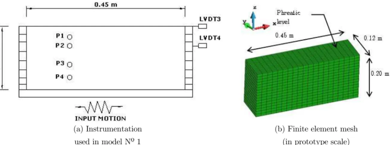
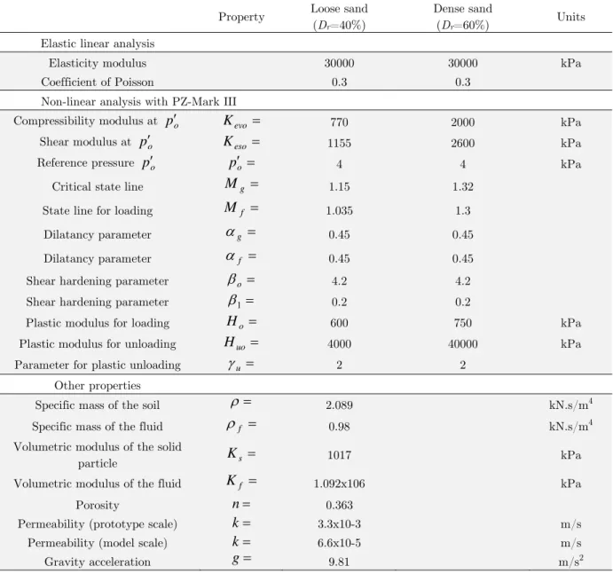
Lique-faction Problems) project is considered. The experiment carried out by Taboada and Dobry (1993) consists of a 0.20 m high, horizontal, uniform Nevada sand layer, which is placed in a laminar box at a relative density of about 40% (loose sand). The purpose of the laminar box is to simulate the response of a semi-infinite loose sand layer during shaking. A sketch of the laminar box and the instrumentation used for this experiment is presented in Figure 1(a). Material properties are listed

in Table 1 (see loose sand column with relative density Dr= 40%). The experiment was carried out

(a) Instrumentation used in model Nº 1

(b) Finite element mesh (in prototype scale)

Figure 1: Geometry and mesh of the finite element model

-0.3 -0.2 -0.1 0 0.1 0.2 0.3

0 5 10 15 20 25

Ac

ce

le

ra

tion

(m

/s

2) x

g

Time (s)

Figure 2: Horizontal input motion at bottom.

Numerical modeling is done in model scale using a three dimensional formulation with a

plane-strain condition. For this purpose, lateral faces at the xz plane are allowed only to move in its

plane. Due to symmetry, only half of the model is considered. The finite element mesh is composed of 5120 coupled hexahedral finite elements with 8-node for pore pressure and 8-node for solid dis-placements (called here 8-8 node elements). The number of degrees of freedom to solve is 24276. The mesh is regular and uniform as shown in Figure 1(b). The laminar box is modeled with the constraint of the lateral tied nodes. The displacements of nodes located at the two ends of the soil at the same level are restrained to have the same value. The base nodes are fixed in both horizontal and vertical directions. Dissipation of pore pressure is allowed only through the top surface of the layer; the lateral boundaries and the base are kept impermeable. The maximum size of a finite ele-ment in the mesh is limited to L



₅1 ₈1



V_s /f in order to permit good wave transmission within

the model, where Vs is the shear wave velocity of the soil and f is the predominant frequency of

loading. The limitation in the xy plane is more flexible and the subdivision in this plane can be

coefficient of



5% and with a circular frequency of loading



2



f .First a static analysis due to application of gravity (model’s own weight) is performed before seismic excitation. The resulting fluid hydrostatic pressures and stress-states along the soil mass are used as initial conditions for the subsequent dynamic analysis (Ou and Chan, 2006).The magnified deformed mesh and excess pore pressure at the end of the analysis are shown in Figures 3(a)-(b), respectively. In Figures (4)-(5) are compared the development of the excess pore pressure at points P1, P2 and P3, P4, (see locations in Figure 1(a)), respectively, as predicted by the present numerical model and those recorded in the experiment. In Figure 6, the lateral displacement at locations LVDT3 and LVDT4 are also depict-ed. As it can be seen, a reasonable good agreement between numerical and experimental results is shown.

Property Loose sand

(Dr=40%)

Dense sand

(Dr=60%) Units

Elastic linear analysis

Elasticity modulus 30000 30000 kPa

Coefficient of Poisson 0.3 0.3

Non-linear analysis with PZ-Mark III

Compressibility modulus at p_o Kevo  770 2000 kPa

Shear modulus at p_o K_eso  1155 2600 kPa

Reference pressure p_o po  4 4 kPa

Critical state line Mg  1.15 1.32

State line for loading Mf  1.035 1.3

Dilatancy parameter



g  0.45 0.45

Dilatancy parameter



f  0.45 0.45

Shear hardening parameter



o  4.2 4.2

Shear hardening parameter



₁ 0.2 0.2

Plastic modulus for loading Ho  600 750 kPa

Plastic modulus for unloading Huo  4000 40000 kPa

Parameter for plastic unloading



u  2 2

Other properties

Specific mass of the soil



 2.089 kN.s/m4

Specific mass of the fluid



f  0.98 kN.s/m4

Volumetric modulus of the solid

particle Ks  1017 kPa

Volumetric modulus of the fluid Kf  1.092x106 kPa

Porosity n 0.363

Permeability (prototype scale) k  3.3x10-3 m/s

Permeability (model scale) k  6.6x10-5 m/s

Gravity acceleration g 9.81 m/s2

a) Deformed mesh (m) b) Excess pore pressure (kPa)

Figure 3: Deformation and excess of pore pressure after 16.38 s.

-10 -5 0 5 10 15 20 25 30

0 2 4 6 8 10 12 14 16

Ex

ce

ss

o de

p

oro

pr

ess

ão (KPa

)

Time (s) P2

Present analysis

Experimental (Taboada and Dobry ,1993)

-10 -5 0 5 10 15 20 25 30

0 2 4 6 8 10 12 14 16

Ex

ce

ss

p

or

e pr

ess

ur

e

(kPa

)

Time (s) P1

Present analysis

Experimental (Taboada and Dobry ,1993)

Figure 4: Excess pore pressure histories for P1 and P2.

-10 0 10 20 30 40 50 60

0 2 4 6 8 10 12 14 16

Ex

ces

so de

por

opre

ssão (KP

a)

Time (s) P4

Present analysis

Experimental (Taboada and Dobry ,1993)

-10 0 10 20 30 40 50 60

0 2 4 6 8 10 12 14 16

Ex

ces

s por

e pre

ssure

(kPa

)

Time (s) P3

Present analysis

Experimental (Taboada and Dobry ,1993)

-0.10 -0.05 0.00 0.05 0.10

0 2 4 6 8 10 12 14 16

De

slo

camento

hor

iz

on

ta

l (

m

)

Time (s) LVDT4

Present analysis

Experimental (Taboada and Dobry ,1993)

-0.10 -0.05 0.00 0.05 0.10

0 2 4 6 8 10 12 14 16

Horiz

ont

al

di

spl

acemen

t (m)

Time (s) LVDT3

Present analysis

Experimental (Taboada and Dobry ,1993)

Figure 6: Lateral displacement for LVTD3 and LVDT4.

Cycles of shear stress-strain histories for different depths in the soil mass are shown in the left part of Figure 7. The shear stress



h refers to the shear stress component



xzacting in the plane

perpendicular to the longitudinal movement due to shaking, while



h is the associated shear

defor-mation component



xz. As it may be observed, the shear deformation reaches a maximum value

around 1.5%. Similarly, the right part of Figure 7 shows the associated shear stress-effective vertical stress paths in the soil mass. As it may be observed, soils at depths 2.81 m and 5.31m are in a liq-uefied state because the effective vertical stresses has almost reduced to zero at the end of shaking.

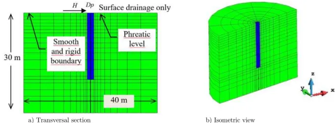
3.2 Soil-Pile System Under Consolidation Load (Taibet and Carter, 2001)

In Taibet and Carter (2001) is studied the time-dependent behavior of a vertical pile inserted in a saturated soil mass and which is submitted to a lateral loading H at its head. In the mentioned reference, a semi-analytical finite element method based on discrete and continuous Fourier trans-formations was used for the analysis of the saturated porous media. The pile diameter is D_p 2.0m and this is inserted in a non-cohesive saturated soil deposit that follows the Mohr-Coulomb law.

The influence of the dilatancy angle



in the soil and pile response was studied by the authors

2.81 m

-12.0 -8.0 -4.0 0.0 4.0 8.0 12.0

-2.0 -1.0 0.0 1.0 2.0

h

(k

Pa

)

γh(%)

2.81 m

-12.0 -8.0 -4.0 0.0 4.0 8.0 12.0

-30 -25 -20 -15 -10 -5 0

h

(k

Pa

)

'v(kPa)

5.31 m

-12.0 -8.0 -4.0 0.0 4.0 8.0 12.0

-2.0 -1.0 0.0 1.0 2.0

h

(k

Pa)

γh(%)

5.31 m

-12.0 -8.0 -4.0 0.0 4.0 8.0 12.0

-60 -50 -40 -30 -20 -10 0

h

(k

Pa

)

'v(kPa)

7.81 m

-16.0 -12.0 -8.0 -4.0 0.0 4.0 8.0 12.0 16.0

-2.0 -1.0 0.0 1.0 2.0

h

(k

Pa

)

γh(%)

7.81 m

-16.0 -12.0 -8.0 -4.0 0.0 4.0 8.0 12.0 16.0

-80 -60 -40 -20 0

h

(k

Pa

)

'v(kPa)

a) Transversal section b) Isometric view

Figure 8: Geometry, boundary conditions and finite element mesh

Material Property Units

Soil

Specific weight ( s) 17 kN/m3

Elasticity modulus (Es ) 30000 kPa

Coefficient of Poisson (νs) 0.3

Cohesion c 0.0 kPa

Friction angle (Ф’ ) 30 o

Dilatancy angle (Ψ) 0 (non-associative) or 30 (associative) o

Permeability (k) 1x10-4 m/s

Fluid specific weight ( f ) 10 kN/m3

Concrete

Specific weight ( c) 23 kN/m3

Elasticity modulus (Ec ) 30x106 kPa

Coefficient of Poisson

( ) 0.2

Table 2: Material properties.

The finite element mesh is formed by 996 20-8 node hexahedral finite elements (20 nodes for the solid phase and 8 nodes for the fluid one) for simulating the saturated soil and 84 20-node hexahe-dral elements for modeling the concrete pile. The number of equations to solve is 16032. In order to provide a direct comparison with the results provided by Taiebat and Carter (2001), all obtained results are expressed in terms of a dimensional time T_v k(1v_s)E_st



_f(12v_s)(1v_s)D_p2 , load

rate d



H fDp



dTv

3

/





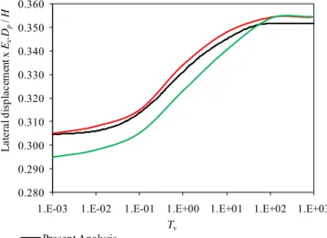
 and pile diameter Dp.

An elastic analysis of the problem was first conducted to evaluate the accuracy of the present

con-stant with time (ramp load). The predicted lateral displacement of the pile head in the direction of

the applied load is plotted against the dimensionless time,

T

v in Figure 9. Results of the analysis

using the discrete and continuous Fourier series method suggested by Taiebat and Carter (2001) are also shown for comparison. As it may be observed, the results of the analysis using the discrete Fourier approach are in close agreement with the results obtained in the present analysis.

0.280 0.290 0.300 0.310 0.320 0.330 0.340 0.350 0.360

1.E-03 1.E-02 1.E-01 1.E+00 1.E+01 1.E+02 1.E+03

La

te

ra

l d

isp

la

ce

m

en

t x

Es

.D

p

/

H

Tv Present Analysis

Discrete Fourier Aproximation (Taiebat and Carter, 2001) Continuous Fourier Aproximation (Taiebat and Carter, 2001)

Figure 9: Lateral displacement at pile head

Secondly, in a series of elasto-plastic analysis, the total lateral load was varied from

3

5 fDp

H 



to H 60



fD3p, where



f is the specific weight of the water . In each case the total

load was applied during a time interval of

T

v



0

.

0001

, with a loading rate of





100000

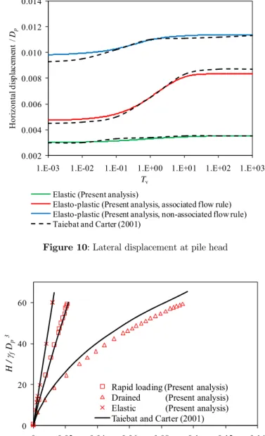
. This

loading rate was sufficiently high to approximate an initial undrained loading. Thereafter, the load was held constant in time and the analysis was continued, allowing excess pore pressures to dissi-pate, and thus for the soil to consolidate. The time-dependent lateral displacements at the pile head predicted by the elasto-plastic analyses with both associated (dilatancy and friction angles are equal) and non-associated (null dilatancy angle) flow rules are plotted in Figure 10 for the particu-lar case ofH 15



fD3p. The response of the pile in elastic soil is also presented.

In order to permit a direct comparison with the results provided by Taiebat and Carter (2001), the excess pore pressures p are expressed in a non-dimensional formp/





_fD_p



.The distributions of the dimensionless excess pore pressures at the end of rapid loading for H 15



_fD3_p are shown in Figures 12(a)-(b) for the cases of soil with an associated and non-associated flow rule, respectively. The interested reader can compare these distributions with those provided in the work of Taiebat and Carter (2001) and good agreement can be inferred.

0.002 0.004 0.006 0.008 0.010 0.012 0.014

1.E-03 1.E-02 1.E-01 1.E+00 1.E+01 1.E+02 1.E+03

H

or

iz

on

ta

l d

isp

lac

em

en

t /

Dp

Tv Elastic (Present analysis)

Elasto-plastic (Present analysis, associated flow rule) Elasto-plastic (Present analysis, non-associated flow rule) Taiebat and Carter (2001)

Figure 10: Lateral displacement at pile head

0 20 40 60

0 0.02 0.04 0.06 0.08 0.1 0.12 0.14

H /

f

Dp

3

Horizontal displacement / Dp

Rapid loading (Present analysis) Drained (Present analysis) Elastic (Present analysis) Taiebat and Carter (2001)

a) Associated flow rule b) Non-associated flow rule

Figure 12: Dimensionless excess pore pressure close to the pile

3.3 Soil-Pile System Under Harmonic Load (Abdoun, 1997)

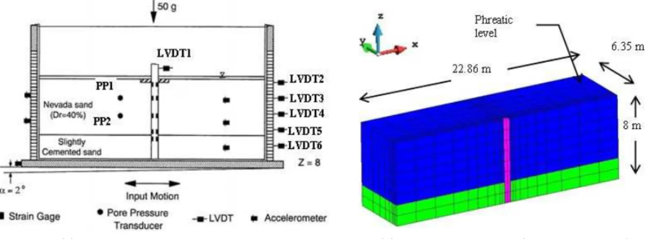
In the centrifuge test reported by Abdoun (1997), a single pile model (called model No 3 in the

ex-perimental work) was embedded in a saturated soil deposit and submitted to a lateral movement at its base. The experiment was conducted using the rectangular, flexible-wall laminar box container shown in Figure 13(a). The soil profile consists of two layer of fine Nevada sand saturated with

water: a top liquefiable layer of relative density, Dr = 40% and 6 m prototype thickness, and a

bot-tom slightly cemented non-liquefiable sand layer with a thickness of 2 m. According to the experi-mental work, the cemented non-liquefiable sand layer has similar properties of a non-liquefiable sand layer with Dr = 60%. Material properties are listed in Table 1. The prototype single pile is 0.6 m in diameter, 8 m in length, has a bending stiffness, EI = 8000 kN.m2, and is free at the top. The

model has an inclination angle of 2o (model scale) and is subjected to the predominantly 2Hz

har-monic base excitation shown in Figure 14 with a peak acceleration of 0.3g, where g is the gravity

acceleration.

and upslope boundaries were tied together (both horizontally and vertically) to reproduced a 1D shear beam effect, (iii) the soil surface was traction free, with zero prescribed pore pressure, and (iv) the base and lateral boundaries were impervious. A static application of gravity (model own weight) was performed before seismic excitation. The resulting fluid hydrostatic pressures and soil stress-states served as initial conditions for the subsequent dynamic analysis. The Rayleigh damping ma-trix was used with a damping coefficient of



5%.

(a) Instrumentation used in model 3 (b) Finite element mesh (in prototype scale)

Figure 13: Geometry and mesh of the finite element model.

-0.4 -0.3 -0.2 -0.1 0 0.1 0.2 0.3 0.4

0 5 10 15 20 25

Ac

ce

le

ra

tio

n

(m

/s

2) x

g

Time (s)

Figure 14: Movement at base (Abdoun 1997).

With a mild inclination of 2o, model 3 attempts to simulate an infinite slope subjected to

As it can be seen, liquefaction was reached down to a depth of 5.0 m (see Figure 15(b)), as indicat-ed by the pore-pressure ratio ru approaching to 1.0 (ru =



p

/

 

v where p is the excess pore

pres-sure and

 

v is the initial effective vertical stress). The Nevada sand layer remained liquefied until

the end of shaking and beyond. Thereafter, excess pore pressure started to dissipate.

The mild inclination of model 3 also imposed a static shear stress component (due to gravity), causing accumulated cycle-by-cycle lateral deformation. The recorded and computed short-term and long-term excess pore pressure histories for two control points (PP1 and PP2) at depths of 1 m and 5 m are compared in Figure 16 and Figure 17, respectively. Both computed and recorded results displayed a number of instantaneous sharp pore pressure drops after initial liquefaction. The numer-ical results obtained in the works of Lu et al. (2004) and Valsamis (2008) are also depicted for com-parison.

(a) Deformed mesh (m)

(b) Potential of liquefaction (ru)

Figure 15: Finite element results at the end of shaking.

-10 -5 0 5 10 15

0 5 10 15 20 25

Ex

cess of po

re

pre

ssure (kP

a)

Time (s)

PP1 (1.0 m)

Present analysis Lu et al. (2004) Experimental Valsamis (2008)

Initial efective vertical stress

-10 0 10 20 30 40 50 60

0 5 10 15 20 25

Ex

cess of pore

pressu

re

(k

Pa)

Time (s)

PP2 (5.0 m)

Present analysis Lu et al. (2004) Experimental Valsamis (2008)

Initial efective vertical stress

-10 -5 0 5 10 15

0 10 20 30 40 50 60 70 80

Ex

ce

ss

of

pore p

ress

ur

e

(kPa)

Time (s)

PP1 (1.0 m)

Present analysis Lu et al. (2004) Experimental Valsamis (2008)

Initial efective vertical stress

-10 0 10 20 30 40 50 60

0 10 20 30 40 50 60 70 80

Ex

ce

ss of p

ore

pre

ssure

(kP

a)

Time (s)

PP2 (5.0 m) Present analysis

Lu et al. (2004) Experimental Valsamis (2008)

Initial efective vertical stress

Figure 17: Long-term excess pore pressure time histories of PP1 and PP2

The permanent lateral displacement of the ground surface after shaking is approximately 100 cm. All lateral displacement occurred in the top 6.0 m within the liquefiable sand layer. The top graph in Figure 18 shows the recorded and computed pile lateral displacement at the soil surface during and after shaking. The computed pile lateral displacement increased to 40 cm and decreased to approximately 8 cm at the end of shaking. The bottom slightly cemented sand layer, as indicated in the bottom graph, did not slide with respect to the base of the laminar box. Lateral displace-ments at some other control points in the soil mass are also shown in Figure 18.

Figure19 shows the profile of pile lateral displacements obtained with the present numerical model for the time in which the maximum lateral displacement occurs at the pile head. In the same graph are also depicted the pile displacement predictions according to some simplifying approaches based on the works of Valsamis et al. (2012), Brandenberg (2005), Cubrinovski et al. (2006), Tokimatsu and Asaka (1998), American Petroleum Institute (API, 2005), High Pressure Gas Safety Institute of Japan (HPGS, 2000) and Railway Technical Research Institute (RTR, 1999). All these references have used a methodology based on the subgrade reaction approach (p-y method). As it may be observed, there is a great difference among all methodologies. The closer predictions to the experimental values are due to the works of RTR (1999), API (1995) and Brandenberg (2005).

Because it is true that major liquefaction does not necessarily takes place at the end of the

shaking, in Figure 20 is depicted the liquefaction evolution measured by the ru factor at different

time instants. As it may be observed, a dilatation zone appears close to the pile head (blue color zones). At the end of the shaking (after 25 seconds of analysis), liquefaction almost took place in the top liquefiable sand layer, thus reflecting a similar condition as established in the experimental work (Lu et al., 2004).

-0.20 0.00 0.20 0.40 0.60 0.80 1.00

0 5 10 15 20 25

Horizontal di splac em ent ( m ) Time (s)

LVDT1 (Pile head) Present analysis

Lu et al. (2004) Experimental Valsamis (2008) -0.20 0.00 0.20 0.40 0.60 0.80 1.00 1.20

0 5 10 15 20 25

Horiz onta l d ispla ce me nt (m) Time (s)

2.0 m (close to LVDT3 (2.5 m)) Present analysis

Lu et al. (2004) Experimental Valsamis (2008) -0.20 0.10 0.40 0.70 1.00 1.30 1.60

0 5 10 15 20 25

H oriz onta l displac em ent ( m ) Time (s)

Surface (close to LVDT2 (0.25 m)) Present analysis

Lu et al. (2004) Experimental Valsamis (2008) -0.20 0.00 0.20 0.40 0.60 0.80 1.00 1.20

0 5 10 15 20 25

Hor iz ont al d isp lace m ent (m ) Tempo (seg.)

4.0 m (close to LVDT4 (3.75 m)) Present analysis

Lu et al. (2004) Experimental Valsamis (2008) -0.08 -0.06 -0.04 -0.02 0.00 0.02 0.04 0.06 0.08

0 5 10 15 20 25

Hor iz ontal displa ce ment (m) Time (s)

LVDT5 (6.0 m) Present analysis

Lu et al. (2004) Experimental Valsamis (2008)

-8 -6 -4 -2

0 0 0.2 0.4 0.6 0.8 1

Dept

h

(m

)

Horizontal displacement (m) Present analysis Valsamis et al. (2012) Brandenberg (2005) Experimental API (1995) HPGS (2000) RTR (1999)

Cubrinovski et al. (2006) Tokimatsu and Asaka (1998)

Figure 19: Profile of pile lateral displacements

1.25 s 2.5 s

5 s 7.5 s

10 s 12.5 s

15 s 16.5 s

20 s 25 s

Figure 22 shows the shear stress- effective vertical stress paths during shaking for the soil zones located in the near field and free-field. As it may be inferred from the graphs, all soil samples have an initial effective vertical stress and a static shear stress value as a result of the initial conditions of the soil (gravity load) and due to the surface inclination. During shaking the effective vertical stress is almost reduced to zero for various soil depths due to soil liquefaction.

1.50 m (Near-field)

-10.0 -5.0 0.0 5.0 10.0 15.0

-10.0 0.0 10.0 20.0 30.0

h

(k

Pa

)

γh(%)

1.50 m (Free-field)

-10.0 -5.0 0.0 5.0 10.0 15.0

-5.0 0.0 5.0 10.0 15.0 20.0 25.0

h

(k

Pa

)

γh(%)

3.50 m (Near-field)

-15.0 -10.0 -5.0 0.0 5.0 10.0 15.0 20.0

-5.0 0.0 5.0 10.0 15.0 20.0

h

(k

Pa

)

γh(%)

3.50 m (Free-field)

-15.0 -10.0 -5.0 0.0 5.0 10.0 15.0 20.0

-5.0 0.0 5.0 10.0 15.0 20.0 25.0

h

(k

Pa

)

γh(%)

5.50 m (Near-field)

-10.0 -5.0 0.0 5.0 10.0 15.0 20.0 25.0

-5.0 0.0 5.0 10.0 15.0 20.0

h

(k

Pa

)

γh(%)

5.50 m (Free-field)

-10.0 -5.0 0.0 5.0 10.0 15.0 20.0 25.0

-5.0 0.0 5.0 10.0 15.0 20.0

h

(k

Pa

)

γh(%)

1.50 m (Near-field)

-10.0 -5.0 0.0 5.0 10.0 15.0

-20 -15 -10 -5 0

h

(k

Pa

)

'v(kPa)

1.50 m (Free-field)

-10.0 -5.0 0.0 5.0 10.0 15.0

-20 -15 -10 -5 0

h

(k

Pa

)

'v(kPa)

3.50 m (Near-field)

-15.0 -10.0 -5.0 0.0 5.0 10.0 15.0 20.0

-40 -30 -20 -10 0

h

(k

Pa

)

'v(kPa)

3.50 m (Free-field)

-15.0 -10.0 -5.0 0.0 5.0 10.0 15.0 20.0

-40 -30 -20 -10 0

h

(k

Pa

)

'v(kPa)

5.50 m (Near-field)

-10.0 -5.0 0.0 5.0 10.0 15.0 20.0 25.0

-60 -50 -40 -30 -20 -10 0

h

(k

Pa

)

'v(kPa)

5.50 m (Free-field)

-10.0 -5.0 0.0 5.0 10.0 15.0 20.0 25.0

-60 -50 -40 -30 -20 -10 0

h

(k

Pa

)

'v(kPa)

Figure 22: Shear stress-vertical effective stress paths in the soil at 1.5 m, 3.5 m, and 5.5 m depths

3.4 Soil-Structure Interaction Examples Under Harmonic Load

they are joined together by a concrete cap. The soil domain is defined by a region of 41.5 m x 30.5 m x 14m along the x, y and z directions, respectively. The typical story height of the steel frame is 3

m and this story is composed of three and two spans of 3.25 m each one along the x and y

direc-tions, respectively. The finite element mesh used in the analysis is shown in Figure 23 and it is formed by 1380 8-node hexahedral finite elements for modeling the pile and cap, 15816 8-8 node hexahedral finite elements for modeling the soil domain, 230 8-node quadrilateral zero-thickness contact elements for modeling the soil-pile interface and 228 2-node truss elements for modeling the steel frame. A half mesh configuration is used due to symmetry considerations and the number of degrees of freedom to solve is 77980. The structural steel properties used in the computations

corre-spond to a W13x426 section with a specific weight of 7.8 kN/m3. In order to show liquefaction, the

soil mass is considered to be composed of a uniform liquefiable sand layer with a relative density Dr

= 40% (see Table 1). The load is applied at the base of the model by using the E-W component of the Centro earthquake (1940) as shown in Figure 24. The predominant frequency of the earthquake is 2Hz and the damping ratio for the Rayleigh damping matrix is 5%. The boundary conditions used in the example of section 3.3 are also used here.

a) Isometric view of soil-frame system b) Plane xz c) Plane yz

Figure 23: Finite element mesh for soil-steel frame system

-0.25 -0.2 -0.15 -0.1 -0.05 0 0.05 0.1 0.15 0.2 0.25

0 5 10 15 20 25 30

Accel

erat

ion

(m/

s

2) x

g

Time (s)

Figure 24: The Centro Earthquake (1940, E-W component)

In Figure 25 is shown the evolution of the liquefaction potential factor ru for different time

Figure 26 shows the lateral displacement histories at the pile cap and stories of the steel frame. As it may be observed, the maximum lateral displacement at the cap is around 0.10 m. Because the soil zones among piles are almost liquefied and there is not exist a non-liquefiable surface layer, the soil zones surrounding the piles do not provide a rigid lateral support, thus pile lateral displace-ments increase considerably.

a) 2 s b) 4 s

c) 8 s d) 16 s

e) 20 s f) 30 s

Figure 25: Evolution of liquefaction potential according to ru factor

-0.2 -0.15 -0.1 -0.05 0 0.05 0.1 0.15

0.0 5.0 10.0 15.0 20.0 25.0 30.0

H

orizon

tal

d

ispla

cem

en

t (m

)

Time (s) Cap First story Second story

-0.35 -0.25 -0.15 -0.05 0.05 0.15 0.25

0.0 5.0 10.0 15.0 20.0 25.0 30.0

H

orizon

tal

d

ispla

cem

en

t (m

)

Time (s)

Third story Fourth story Fifth story Sixth story

Figure 26: Horizontal displacements at different levels of the structure

a) 4 s (fixed base) b) 4s (flexible base) c) 12 s (fixed base)

d) 12 s (flexible base) e) 20 s (fixed base) f) 20 s (flexible base)

g) 30 s (fixed base) h) 30 s (flexible base)

-1.5 -1 -0.5 0 0.5 1 1.5

0.0 5.0 10.0 15.0 20.0 25.0 30.0

A

xial

fo

rc

e

(k

σ)

Time (s)

Element 1 (fixed base) Element 1 (Flexible base)

-250 -200 -150 -100 -50 0 50 100 150 200 250

0.0 5.0 10.0 15.0 20.0 25.0 30.0

A

xial

fo

rc

e

(k

σ)

Time (s)

Element 2 (Fixed base) Element 2 (Flexible base)

Figure 28: Axial force histories in elements 1 and 2

As it may be observed, the axial forces in these elements are significantly different for the cases of rigid and flexible base support. Thus, for the present example, the soil deposit must be included in the analysis. This result was expected since the soil mass is represented by a loose sand layer, which is not rigid at all.

4 CONCLUSIONS

In this study, a computer program for the three dimensional finite element analysis of soil-structure

systems was developed. The numerical model uses the coupled dynamic field equation with the u-p

formulation of Biot’s theory for modeling saturated soils, while concrete caps and piles are modeled as monophasic materials. The superstructure can be modeled by using shell, solid and beam-column finite elements. The numerical model is firstly validated with some benchmarks found in the tech-nical literature. Detailed comparison between numerical and experimental results for soil and soil-pile systems showed acceptable matching. Also, the numerical model was able to predict dilatation zones close to the pile heads, which characterize soil-pile systems involving liquefaction. Only after validation processes have been successfully completed, the following parametric studies can be done with the aim of the present numerical tool. Numerical modeling and simulation can be used to pre-dict the behavior of piles or pile groups embedded in fully saturated soils and thus used to improve design in terms of safety and economy. When liquefaction is involved in the analysis, a complex constitutive model capable of simulating dilatancy and cyclic mobility in the soil mass was proved to perform well. Potentiality of the numerical tool is shown by modeling a steel frame building sup-ported by a group of concrete piles under seismic load. The obtained results showed that the soil zones among piles have a high potential of liquefaction (ru close to one). Also, axial forces in the steel frame elements are underestimated when the frame is considered to be clamped to the ground directly. Studies are in progress in order to improve the modeling of hysteretic damping in the soil.

Acknowledgments

References

Abdoun T. (1997). Modeling of seismically induced lateral spreading of multi-layered soil and its effect on pile foun-dations. Ph.D. Thesis, Rensselaer Polytechnic Institute, USA.

API (1995). Recommended practice for planning, designing and constructing fixed offshore platform, Washington, DC: American Petroleum Institute

Brandenberg SJ. (2005). Behavior of pile foundations in liquefied and laterally spreading ground. Ph.D. Thesis, Uni-versity of California, Davis, USA.

Chaloulos Y. K., Bouckovalas G.D, Karamitros D. K. (2013a). Pile response in submerged lateral spreads: Common pitfalls of numerical modeling techniques, Soil Dynamics and Earthquake Engineering 55: 275-287

Chaloulos Y. K., Bouckovalas G.D, Karamitros D. K. (2013b). Analysis of liquefaction effects on ultimate pile reac-tion to lateral spreading, Journal of Geotechnical and Geoenviromental Engineering 140: 1-11

Chatterjee K.,Choudhury D., Poulos H.G. (2015). Seismic analysis of laterally loaded pile under influence of vertical loading using finite element method, Computers and Geotechnics 67: 172-186

Cubrinovski M., Kokusho T., Ishihara K. (2006). Interpretation from large-scale shake table tests on piles undergoing lateral spreading in liquefied soils, Soil Dynamics and Earthquake Engineering 26: 275-286

Cuellar, P. (2011). Pile foundations for offshore wind turbines: numerical and experimental investigations on the behavior under short-term and long-term cyclic loading. Ph.D. Thesis. Berlin:Technischen Universitat, Germany Gu Q., Yan Z., Peng Y. (2016). Parameters affecting laterally loaded piles in frozen soils by an efficient sensitivity analysis method, Cold Regions and Technology 121:42-51

High Pressure Gas Safety Institute of Japan (2000). Design method of foundation for level 2 earthquake motion (In Japanese)

Jeremic B. (2004). Domain reduction method for soil-foundation-structure interaction analysis. Technical Report UCD-CGM 01-2004.

Khodair Y., Mohti A. (2014). Numerical analysis of pile-soil interaction under axial and lateral loads, International Journal of Concrete Structures and Materials 8: 239-249

Kumari S., Sawant V. A. (2013). Use of infinite elements in simulating liquefaction phenomenon using coupled ap-proach, Coupled Systems Mechanics 2: 375-387

Leung K. H. (1984). Earthquake response of saturated soil and liquefaction, Ph.D. Thesis, University College of Swansea, UK

Lewis R. W., Schrefler B. A. (1998). The Finite Element Method in the Static and Dynamic Deformation and Con-solidation of Porous Media (2th Edition). John Wiley and Sons Ltd (New York).

Lu J., He L., Yang Z., Abdoun T., Elgamal A. (2004). Three dimensional finite element analysis of dynamic pile behavior in liquefied ground. In: Doolin D, Kammerer A, Nogami T, Seed R, eds. Proceedings of the 11th Interna-tional Conference on Soil Dynamics and Earthquake Engineering(11ICSDEE), Berkeley, United States

Maheshwari B. K., Sarkar, R. (2011). Seismic behavior of soil-pile structure interaction in liquefiable soils: paramet-ric study, International Journal of Geomechanics 11: 335-347

McGann C. R., Arduino P., Mackenzie-helnwein P. (2012). Stabilized single-point 4-node quadrilateral element for dynamic analysis of fluid saturated porous media, Acta Geotechnica 7: 297-311

Ou J. H., Chan A. H. C. Three dimensional numerical modeling of dynamic saturated soil and pore fluid interaction. In: Topping B H V, Montero G, Montenegro R, eds. Proceedings of the Fifth International Conference on Engineer-ing Computational Technology, StirlEngineer-ingshire, United KEngineer-ingdom, 2006

Railway Technical Research Institute (1999), Earthquake resistant design code for railway structures, Maruzen Co. (In Japanese)

Taboada V. M, Dobry R. (1993). Experimental results and numerical predictions of model No 1. In: Arulanandan K, Scott R F, eds. Proceedings of the International Conference on the Verification of Numerical Procedures for the analysis of soil liquefaction problems, California, United States.

Taiebat H.A., Carter J.P. (2001). A semi-analytical finite element method for three-dimensional consolidation analy-sis, Computers and Geotechnics 28:55-78

Tamayo J. L. P. (2015). Numerical simulation of soil-pile interaction by using the finite element method. Ph.D. Thesis. Federal University of Rio Grande do Sul, Brazil.

Tamayo J. L. P.,Morsch I.B, Awruch A. M. (2013). Static and dynamic analysis of reinforced concrete shells, Latin American Journal of Solids and Structures 10: 1109-1134

Tasiopoulou P., Taiebat M., Tafazzoli N. (2015a). On validation of fully coupled behavior of porous media using centrifuge test results, Coupled Systems Mechanics 4:37-65

Tasiopoulou P., Taiebat M., Tafazzoli N. (2015b). Solution verification procedures for modeling and simulation of fully coupled porous media: static and dynamic behavior, Coupled Systems Mechanics 4:67-98

Tokimatsu K., Asaka Y. (1998). Effects of liquefaction-induced ground displacements on pile performance in the 1995 Hyogoken-Nambu earthquake, Soil and Foundations, Special Issue: 163-177

Valsamis A. I (2008). Numerical simulation of single pile response under liquefaction induced lateral spreading. Ph.D. Thesis. Department of Geotechnical Engineering, School of Civil Engineering, National Technical University of Ath-ens, Greece.

Valsamis A. I, Bouckovalas G. D, Chaloulos Y. K. (2012). Parametric analysis of single pile response in laterally spreading ground, Soil Dynamics and Earthquake Engineering 34: 99-110