Anisotropic Probabilistic Cellular Automaton for a Predator-Prey System
Kelly C. de Carvalho and Tˆania Tom´e Instituto de F´ısica, Universidade de S˜ao Paulo
Caixa Postal 66318 05315-970 S˜ao Paulo, SP, Brazil
Received on 13 April, 2007
We consider a probabilistic cellular automaton to analyze the stochastic dynamics of a predator-prey system. The local rules are Markovian and are based in the Lotka-Volterra model. The individuals of each species reside on the sites of a lattice and interact with an unsymmetrical neighborhood. We look for the effect of the space anisotropy in the characterization of the oscillations of the species population densities. Our study of the probabilistic cellular automaton is based on simple and pair mean-field approximations and explicitly takes into account spatial anisotropy.
Keywords: Cellular automata; Predator-prey systems; Spatial models; Spatio-temporal patterns; Mean-field approach
I. INTRODUCTION
In the last years a particular great effort has been done in or-der to unor-derstand the role of space given by a spatial structure and local interactions in the characterization of the dynam-ics of competing biological species systems [1–18]. In this context it has been studied irreversible stochastic lattice mod-els [19–21] with the purpose of mimic predator-prey systems with Markovian local rules based in the Lotka-Volterra model [22, 23]. One of the problems that has been object of study is the connection between the time oscillations of population densities and spatial pattern distribution of the individuals of each species.
Here we study the coexistence of a two-species system by considering a probabilistic cellular automaton (PCA) which is a modified version of the automaton devised in [10, 14, 17, 18]. The model, to be called anisotropic predator-prey PCA possess local rules that are similar to the ones of the cellular automaton proposed in [24] and was introduced by us in or-der to explore the effect of spatial anisotropy in the temporal oscillations.
We report dynamic mean-field approximations which take into account the spatial dependence of densities and pair cor-relations of sites. In the next section we present the model. In Sec. 2 we show the equations for the time evolution of species densities and show the spatial dependence of these equations. In Sec. 3 and 4 we perform dynamic simple and pair mean-field approximations. Last section summarize the model, method and results.
II. MODEL
The physical space occupied by the species is represented by a regular lattice ofNsites in which each site can be in one of three states. At each site of the lattice we attach a stochastic variableηithat takes the values 0, 1 and 2 according whether the sitei is empty, or occupied by a prey or occupied by a predator, respectively. The state of the system can be repre-sented by the vectorη= (η1,η2, . . . ,ηN). The time evolution equation forPℓ(η), the probability of stateηat timeℓ, is given
2
b
c
1
0
a
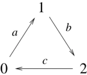
FIG. 1: Transitions of the predator-prey model. The three states are: prey (1), predator (2) and empty (0). The allowed transitions obey the cyclic order shown.
by
Pℓ+1(η) =
∑
σ′
W(η|η′)Pℓ(η′) (1)
where the sum is over the 3Nconfigurations of the system and W(η|η′)is the transition probability from a stateη′to stateη, given that at the previous time step the system was in stateη′.
Since we are considering probabilistic cellular automata, all the sites are updated simultaneously. In this case we have
W(η|η′) =
N
∏
i=1wi(ηi|η′) (2)
wherewi(ηi|η′) is the conditional transition probability per
site.
A. The anisotropic predator-prey PCA
The stochastic rules, embodied in the transition rate wi(ηi|η′), are set up in order that the allowed transitions
C
N
E
n
+1
+2
n
n
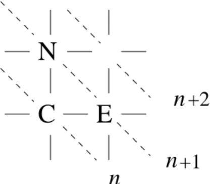
FIG. 2: A site (C) of the square lattice and its two nearest neighbor sites to the east (E) and to the north (N). The layers,n,n+1,n+2, ... are perpendicular to the southwest-northeast direction.
The anisotropic predator-prey PCA has three parameters:a, the probability of birth of prey,b, the probability of birth of predator and death of prey, andc, the probability of predator death. Two of the process are catalytic: the occupancy of a site by prey or by a predator is conditioned, respectively, to the existence of prey or predator in the neighborhood of the site. The third reaction, where predator dies, is spontaneous, that is, it occurs, with probabilityc, independently of the neighbors of the site. We assume thata+b+c=1 with 0≤a,b,c≤1.
The transition probabilities of the anisotropic predator-prey PCA are described in what follows:
(a) If a siteiis empty,ηi=0, and if at north or east there is at least one prey, then it can be occupied by a prey,ηi=1, in the next time step, with a probability proportional to the parameteraand to the number of preynaat north and east of
sitei.
(b) If a site is occupied by a prey,ηi=1, then the site has a probability of being occupied by a new predator,ηi=2, in the next time step if there are prey at north or east. In this process the prey dies instantaneously. The transition proba-bility is proportional to the parameterb and the number of predators at north and east of sitei.
(c) If siteiis occupied by a predator,ηi=2, it dies sponta-neously with probabilityc.
The anisotropic cellular automaton is a variation of the au-tomaton introduced in [10, 14, 17, 18]. Here each site of a regular square lattice interacts with its first neighbors only at two preferential directions. This anisotropic neighborhood consists of the northern and eastern neighbors of each site as shown in Fig. 2. The set of transition probabilities per site is given by
wi(1|η) = a
2n1δ(ηi,0) + (1− b
2n2)δ(ηi,1), (3) wi(2|η) =
b
2n2δ(ηi,1) + (1−c)δ(ηi,2) (4) and
wi(0|η) = (1−
1
2an1)δ(ηi,0) +cδ(ηi,2) (5) where
n1=
∑
kδ(ηk,1) and n2=
∑
kδ(ηk,2) (6)
and the sum is over the neighbor sites localized at east and north of siteiand correspond to the number of neighbors of siteioccupied by prey individuals and predators individuals, respectively.
We have considered this probabilistic cellular automaton with the purpose of verifying the effect of anisotropy in the properties of the time oscillations of the predator-prey system. The rules considered are in some sense inspired in the north-east-center (NEC) cellular automaton [24], which also con-sider an unsymmetrical neighborhood of northern and eastern sites.
The present stochastic dynamics predicts the existence of states, called absorbing states, in which the system becomes trapped. Once the system has entered such a state it cannot es-cape from it anymore remaining there forever. There are two absorbing states. One of them is the empty lattice. The other absorbing state is the one in which the lattice is full of prey. This situation occurs if there are few predators and they be-come extinct. The remaining prey will then reproduce without predation filling up the whole lattice. The existence of absorb-ing stationary states is an evidence of the irreversible character of the model or, in other words, of the lack of detailed balance [21]. However, the most interesting states, the ones that we are concerned with in the present study, are the active states characterized by the coexistence of prey and predators.
B. Evolution equation for state functions
The densities of prey, predator and empty sites are defined as
Piℓ(1) =hδ(ηi,1)iℓ, (7)
Piℓ(2) =hδ(ηi,2)iℓ, (8)
Piℓ(0) =hδ(ηi,0)iℓ, (9) respectively. The lower indexiis used to denote the site and the upper indexℓstands for the time. The pair correlation of two neighbor sitesiand jone being occupied by prey and the other by predator is defined as
Pi jℓ(1 2) =hδ(ηi,1)δ(ηj,2)iℓ. (10) In this definition the sitesiandjare two neighboring horizon-tal sites, the site jbeing at the east ofi. For two neighboring sites placed vertically we use the notation
Pikℓ
µ
2 1
=hδ(ηi,1)δ(ηj,2)iℓ, (11) wherekdenotes the neighbor ofito the north.
Pi′(1) =a
2
·
Pi j
µ
1 0
+Pik(0 1)
¸
+Pi(1)− b 2
·
Pi j
µ
2 1
+Pik(1 2)
¸
, (12)
where we have used prime and unprimed to denote quantities at timeℓ+1 andℓ, respectively. Again,Pi j(10)denotes a pair
correlation of a siteiwhich is empty and its neighbor at the northjwhich is occupied by a prey andPik(0 1)denotes the
pair correlation of the siteiwhich is is empty and its neighbor to the eastkwhich is occupied by a prey. Note that siteiis the site to be updated. The time evolution equation for the density of predators at siteiis given by
Pi′(2) =b
2
·
Pi j
µ
2 1
+Pik(1 2)
¸
+ (1−c)Pi(2). (13)
The evolution equations for correlations of two neighbor sites are given by equations which involves clusters of two, three and four neighbors to the north and east and they are too cumbersome. We will write them in the pair approximation in the next subsection.
We will assume in the present analysis that the densities and the pair correlations are homogeneous so that the correla-tions of sites placed horizontally or vertically are the same. In other words the systems exhibits a specular symmetry along the southwest-northeast line (see Fig. 2). Therefore,
Pi jℓ
µ
1 0
=Pikℓ(0 1) (14)
and
Pi jℓ
µ
2 1
=Pikℓ(1 2). (15)
III. SIMPLE MEAN-FIELD APPROXIMATION
We will first analyze the equations (12) and (13) for the densities of prey and predators by means of a simple mean field approximation [21, 26, 27]. In this approximation we write the probability of a given cluster of sites as the product of the probabilities of each site. In our analysis we maintain the space dependence of each probability. This is necessary since the rules that define the model are not isotropic. We will use the notations
xn=Pn(1), yn=Pn(2) zn=Pn(0). (16)
where the indexnstands for a site at thenlayer. A layer is defined as the sites belonging to a line perpendicular to the southwest-northeast axis, as shown in Fig. 2. Using this ap-proximation and considering equations (12) and (13) we ob-tain
x′n=aznxn+1+xn−bxnyn+1, (17)
and
y′n=bxnyn+1+ (1−c)yn. (18)
wherezn=1−xn−yn. Due to this relation there is no need
for the equation for the density of empty sites.
The analysis of the above set of equations show that the sta-ble solutions are of two types: a prey absorbing state, where the all lattice is full of prey; and an active solution with prey and predators densities constant in time and space. So, we have just homogeneous and nonoscillating solutions when we treat the anisotropic PCA by means of simple mean-field ap-proximation. At this level of mean-field approximation the space anisotropy does not play any role in determining the kind of coexistence of species.
IV. PAIR-MEAN FIELD APPROXIMATION
Now we consider the evolution equations for one-site cor-relations and two site (pair) corcor-relations. The evolution equa-tions for the pair correlaequa-tions depend on clusters of three and four sites. Following the approach of the pair approximation [25–28] we write the clusters of three and four sites as prod-ucts of pair correlations and one-site correlations. However, we must be careful in doing this approximation because we are maintaining the spatial anisotropy dependence of the one and two site correlations. For example, the correlation of a site at layernin state 0, a site at layern+1 in state 0 and a site at layern+2 in state 1, is written in the pair approximation as
Pn,n+1,n+2(001) =
Pn,n+1(00)Pn+1,n+2(01) Pn+1(0)
. (19)
There are more complex clusters that appear in the evolution equation for pair correlations. For example, the following cluster of four sites is approximated by
Pn,n+1,n+2
µ
2 0 0 1
=Pn,n+1(02)Pn,n+1(00)Pn+1,n+2(01)
Pi(0)Pn+1(0)
. (20)
Now we use the notation
Pn,n+1(01) =un, Pn,n+1(12) =vn, Pn,n+1(02) =wn, (21)
Pn,n+1(10) = fn, Pn,n+1(21) =gn, Pn,n+1(20) =hn, (22)
Pn,n+1(11) =rn, Pn,n+1(22) =sn, Pn,n+1(00) =qn. (23)
0 100 200 300 400 500
n
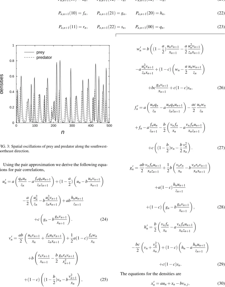
0 0.2 0.4 0.6 0.8 1densities
prey predatorFIG. 3: Spatial oscillations of prey and predator along the southwest-northeast direction.
Using the pair approximation we derive the following equa-tions for pair correlaequa-tions,
un′ =a
µ
qnun zn
−afnqnun+1
znzn+1
+ (1−a 2)
µ
un−b unvn+1
xn+1
−a
2
µu2 n zn
−bu
2 nvn+1 znxn+1
+abhnun+1 zn+1
+c
µ
gn−b gnvn+1
xn+1
. (24)
vn′=ab
2
µ
unvn+1 xn
+ fnunvn+1
znxn+1
+1
2a(1−c) fnwn
xn
+b
Ã
rnvn+1 xn+1 −
b 2
gnrnvn+1 x2n+1
!
+(1−c)
Ã
(1−b 2)vn−b
v2n+1 xn
!
, (25)
wn′=b
µ
(1−a 2)
unvn+1 xn+1 −
a 2
u2nvn+1 znxn+1
−au
2 nvn+1 znxn+1+ (1−
c)
µ
wn− a 2
unwn+1 zn
+bcgnvn+1 xn+1 +
c(1−c)sn, (26)
fn′=a
µu
nqn zn
−aunqnun+1
znzn+1
−ac
2 unwn
zn
+fn−a fnun zn+1−
b 2
µ
vnfn xn
−avnfnun+1
xnzn+1
+c
µ
(1−b 2)vn−
b 2
v2n xn
. (27)
gn′ =ab
2
vnfnun+1 xnzn+1 +
1 2b
µ
vnrn xn
−bvnrnvn+1
xnxn+1
+a(1−c)hnun+1
zn+1
+(1−c)
µ
gn−b gnvn+1
xn+1
, (28)
hn′=b
2
µv
nfn xn
−avnfnun+1
xnzn+1
−bc
2
µ
vn+ v2n xn
+ (1−c)
µ
hn−a hnun+1
zn+1
+c(1−c)sn. (29)
The equations for the densities are
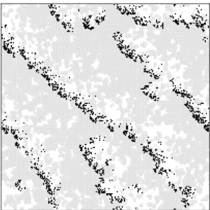
FIG. 4: Snapshot of a configuration obtained from Monte Carlo sim-ulation of the PCA in a square lattice with periodic boundary condi-tions. Predator and prey individual are represented by black and grey points, respectively. The fronts move from northeast to southwest.
and
yn′=bvn+ (1−c)yn. (31)
Therefore, we get a set of eight equations that we have it-erated to find the solutions. We considered periodic boundary conditions and an initial condition where half of the lattice with a set of densities and the other half with another set of densities.
Fora=b and great values of cthe system attains a sta-tionary state which is the absorbing prey state. Decreasingc there is a transition to an active state, coexistence of species, and we found very interesting solutions which are character-ized by travelling waves of the densities of each species. In Fig. 3 we show, for a particular set of the parametersa=b andc=0.05, the prey and predators oscillations as a function of space and for a fixed instant of time. We can see that the behavior of the space oscillations are very complex and very different from a sinusoidal wave.
We remark that our assumption concerning the spatial de-pendence of densities and pair correlations underlying our
mean-field approach could not easily be conceived a priori. It was set up by considering the type of local dynamics with unsymmetrical rules and from the results of Monte Carlo sim-ulations for the present PCA [10, 29]. To further clarify this point we show in Fig. 4 a snapshot generated by simulation of the present PCA on a square lattice where each site can be occupied by prey, predators or can be empty. Periodic bound-ary conditions were used and the system evolved in time ac-cording to the rules defined by Eqs. (3), (4) and (5). A syn-chronous update was used. We see that the distribution of individuals of each species is not homogeneous but exhibits a pattern composed by layers of prey and predators. These lay-ers are displayed in a manner perpendicular to the southwest-northeast direction, the direction along which the oscillations occur as can be seen in Fig. 4. We have found that the spa-tial oscillations do not occur independently of the time oscil-lations, since the spatial layers of prey and predators are not static but are like fronts moving along the southwest-northeast direction. The spatial pattern oscillations are intimately asso-ciated to local time oscillations of the species [10, 29]. These features were incorporated in the present mean-field analysis of the model.
V. CONCLUSIONS
We have considered a predator-prey probabilistic cellular automaton with anisotropic local stochastic rules. We stud-ied this model by means of dynamic mean-field approxima-tion at two orders: simple mean-field approximaapproxima-tion and pair mean-field approximation. Due to the anisotropy these ap-proximations only can be performed if we consider the spatial dependence of probabilities. The simple mean-field approx-imation for this automaton just provides the prey absorbing state and active spatial homogeneous solutions which are also constant in time. The pair mean-field approximation gives much more rich results and show that the active states charac-terized by time oscillations of species densities are inhomoge-neous in space. Therefore, we have spatiotemporal patterns of coexistence. This is in accordance with previous Monte Carlo simulations [10] where we have found local time oscillations connected to inhomogeneous spatial distributions of species individuals.
[1] K. Tainaka, Phys. Rev. Lett.63, 2688 (1989).
[2] R. Durrett and S. Levin, Theor. Popul. Biol.46, 363 (1994). [3] A. Hastings, Population biology: concepts and models,
Springer, New York, 1997.
[4] J. Satulovsky and T. Tom´e, Phys. Rev. E bf 49, 5073 (1994). [5] D. Tilman and P. Kareiva,Spatial ecology: the role of space
in population dynamics and interactions, Priceton University Press, Princeton, 1997.
[6] J. Satulovsky and T. Tom´e, J. Math. Biol.35, 344 (1997). [7] R. Durrett and S. Levin, J. Theor. Biol.205, 201 (2000).
[8] T. Antal and M. Droz, Phys. Rev. E63, 056119 (2001). [9] M. A. M. de Aguiar, H. Sayama, M. Baranger, and Y. Bar-Yam,
Braz. J. Phys.33, 514 (2003).
[10] K. C. de Carvalho and T. Tom´e, Mod. Phys. Lett. B18, 873 (2004).
[11] A. F. Rozenfeld and E. V. Albano, Phys. Lett. A 332, 361 (2004).
[12] D. Chowdhury and D. Stauffer, J. Biosc.30, 277 (2005). [13] G. Szab´o, J. Phys. A38, 6689 (2005).
(2006).
[15] M. Mobilia, I. T. Giorgiev, and U. C. T¨auber, Phys. Rev. E73, 040903 (2006).
[16] S. Morita and K. Tainaka, Popul. Ecol.48, 99 (2006). [17] E. Arashiro and T. Tom´e, J. Phys. A40, 887 (2007)
[18] T. Tom´e and K. C. de Carvalho, Stable oscillations in a predator-prey system: a mean-field approach, arXiv:0704.0512v1 cond-mat stat-mech.
[19] T. M. Liggett, Interacting Particle Systems, Springer, New York, 1985.
[20] J. Marro and R. Dickman,Nonequilibrium Phase Transitions, Cambridge University Press, Cambridge, 1999.
[21] T. Tom´e and M. J. de Oliveira,Dinˆamica Estoc´astica e Irre-versibilidade, Editora da Universidade de S˜ao Paulo, S˜ao Paulo, 2001.
[22] A. Lotka, J. Am. Chem. Soc.42, 1595 (1920); Proc. Nat. Acad. of Sciences USA6, 410 (1920);Elements of Mathematical Bi-ology, Dover, New York (1924).
[23] V. Volterra,Lec¸ons sur la Theorie Math´ematique de la Lutte pour la Vie, Gauthier-Villars, Paris, 1931.
[24] C. H. Bennett and G. Grinstein, Phys. Rev. Lett.55, 657 (1985). [25] R. Dickman, Phys. Rev. A bf 34, 4246 (1986).
[26] T. Tom´e, Physica A212, 99 (1994).
[27] T. Tom´e and J. R. Drugowich de Fel´ıcio, Phys. Rev. E53, 3976 (1996).
[28] T. Tom´e, E. Arashiro, J. R. Drugowich de Fel´ıcio, and M. J. de Oliveira, Braz. J. Phys.33, 458 (2003).