Atmos. Chem. Phys., 10, 3583–3599, 2010 www.atmos-chem-phys.net/10/3583/2010/ © Author(s) 2010. This work is distributed under the Creative Commons Attribution 3.0 License.
Atmospheric
Chemistry
and Physics
Turbulence associated with mountain waves over Northern
Scandinavia – a case study using the ESRAD VHF radar and the
WRF mesoscale model
S. Kirkwood1, M. Mihalikova1, T. N. Rao2, and K. Satheesan1
1Swedish Institute of Space Physics, P.O. Box 812, 98128 Kiruna, Sweden 2National Atmospheric Research Laboratory, Gadanki, India
Received: 6 July 2009 – Published in Atmos. Chem. Phys. Discuss.: 2 October 2009 Revised: 1 April 2010 – Accepted: 8 April 2010 – Published: 16 April 2010
Abstract. We use measurements by the 52 MHz wind-profiling radar ESRAD, situated near Kiruna in Arctic Swe-den, and simulations using the Advanced Research and Weather Forecasting model, WRF, to study vertical winds and turbulence in the troposphere in mountain-wave condi-tions on 23, 24 and 25 January 2003. We find that WRF can accurately match the vertical wind signatures at the radar site when the spatial resolution for the simulations is 1 km. The horizontal and vertical wavelengths of the dominating mountain-waves are∼10–20 km and the amplitudes in verti-cal wind 1–2 m/s. Turbulence below 5500 m height, is seen by ESRAD about 40% of the time. This is a much higher rate than WRF predictions for conditions of Richardson number (Ri)<1 but similar to WRF predictions ofRi<2. WRF
pre-dicts that air crossing the 100 km wide model domain cen-tred on ESRAD has a∼10% chance of encountering con-vective instabilities (Ri<0) somewhere along the path. The
cause of lowRi is a combination of wind-shear at synoptic
upper-level fronts and perturbations in static stability due to the mountain-waves. Comparison with radiosondes suggests that WRF underestimates wind-shear and the occurrence of thin layers with very low static stability, so that vertical mix-ing by turbulence associated with mountain waves may be significantly more than suggested by the model.
1 Introduction
The Scandinavian mountain chain acts as a significant bar-rier to westerly winds from the North Atlantic (see Fig. 1). Winter storm tracks very often bring deep depressions into
Correspondence to:S. Kirkwood ([email protected])
the region and strong westerly winds across the mountain chain are a common result. It is well known that strong winds across mountain chains can lead to the formation of mountain lee waves, and these waves have long been recognised over the Scandinavian mountains (e.g. Larsson, 1954). Mountain waves have been particularly well studied over the mountain chains in western USA, where they can lead to extreme tur-bulence, and more rarely, to aircraft accidents see e.g. (Doyle and Durran, 2002; Doyle and Duran, 2004) and references therein. The Scandinavian mountains are not as high as the mountains of western USA, and there is much less air traffic, so turbulence associated with Scandinavian mountain waves is less important for air-safety. However, turbulence is poten-tially of substantial interest for its role in mixing atmospheric constituents between different heights.
The stratosphere, and the troposphere in high-latitude re-gions, such as Scandinavia, are generally considered to be statically stable (except in sporadic summer thunderstorms). Large scale models which trace air-mass transport, for ex-ample in considering downward transport of ozone from the stratosphere, generally assume no vertical mixing, or a small fixed diffusion coefficient, in these regions (Stohl et al., 2005). Such models find that ozone from the stratosphere contributes very little to ozone concentrations in the lower troposphere (Sprenger and Wernli, 2003; James et al., 2003; Stohl, 2006), in contrast to chemical tracer studies which suggest a much higher contribution (e.g. Dibb et al., 2003).
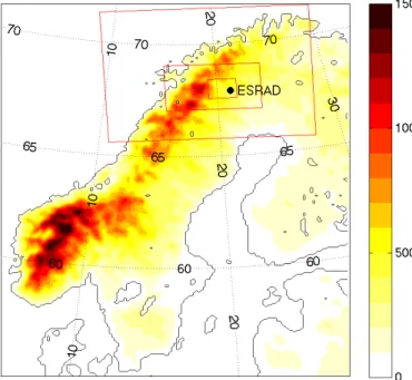
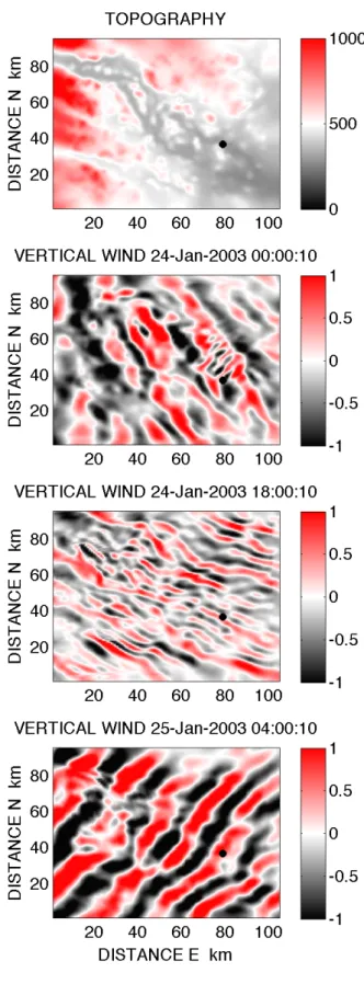
Fig. 1. Map of Scandinavia showing the topography (colour scale with heights in m), the location of the ESRAD radar, and the nested model domains used for the WRF simulations (red rectangles). The outermost domain has horizontal resolution 15 km, the indermediate domain 3 km, and the inner domain around the location of ESRAD has 1 km resolution. Lines of latitude and longitude are shown with dotted lines.
altitudes through isentropic transport, often pass over the Scandinavian mountains (Rao et al., 2008). These are of-ten associated with high-speed westerly winds at the surface, which will lead to mountain waves with the potential for as-sociated turbulence (Rao and Kirkwood, 2005). There is a significant seasonal variation in the occurrence of folds, with a winter maximum (Rao et al., 2008), which is a potential contributing factor to the seasonal variation of ozone in the free troposphere (Rao et al., 2003). There is also an unex-plained seasonal variation in surface ozone in the polar re-gions, with observed wintertime concentrations substantially higher than the values predicted by state-of-the-art models (Tarasova et al., 2007; Zeng et al., 2008). Vertical mixing in association with the winter maximum in tropopause folds might explain this feature, if the mixing is strong enough.
The best available observational method for direct obser-vations of atmospheric turbulence with climatological time coverage is atmospheric radar (see e.g. Wilson, 2004 for a review). Radar observations give a direct estimate of the root mean square (r.m.s) turbulent velocities (in the vertical direc-tion) in air parcels passing overhead of the radar site, and of their temporal variability at that single location. Multi-year statistics of the amount and occurrence rates of turbulence have been published for a number of locations, in the USA, Japan and India (Nastrom et al., 1986; Fukao et al., 1994; Kurosaki et al., 1996; Nastrom and Eaton, 1997, 2005; Rao
et al., 2001). Translating this information to quantitative esti-mates of vertical mixing on a regional scale requires knowl-edge of both the processes causing the turbulence and of the spatial and temporal variability of the turbulence. The studies mentioned above have considered the relationship between turbulence and synoptic weather conditions, but not the rela-tionship to mountain waves, although a statistical correlation between enhanced turbulence and gravity waves was noted by Nastrom et al. (1986).
The ESRAD (ESrange RADar) VHF wind-profiling radar (Chilson et al., 1999) has been in essentially continuous op-eration since late 1996. This radar is situated on the lee side of the Scandinavian mountain chain at 67.9◦
N, 21.1◦ E (see Fig. 1), and often sees the signatures of mountain waves (R´echou et al., 1999). Our aim in this study is to determine whether, with the help of a mesoscale atmospheric model, we can understand the conditions leading to the turbulence which is often seen by the radar in association with moun-tain waves. This is an essential first step to be able to use radar turbulence observations to help quantify the amount of turbulent mixing taking place on a regional and climatologi-cal sclimatologi-cale.
S. Kirkwood et al.: Turbulence and mountain waves 3585 lidar observations from that site. Pluogonven et al. (2008),
modelled mountain waves over the Antarctic peninsula (us-ing a 7 km horizontal resolution). They found horizontal wavelengths 65–80 km and a few m/s amplitude in vertical winds. The model supported the conclusion that turbulence in the lower stratosphere was responsible for the loss of a long-duration balloon as it crossed the area. Oscillations in the float height of second balloon passing nearby provided a reasonable validation of the horizontal wavelength and verti-cal wind amplitude. Generally, for these cases, possibilities to validate the model simulations were limited and there is no way to assess how representative such events are for the locations where they were observed (rather the opposite – the events were studied because of their uniqueness).
A number of studies using 3-D modelling for more typical conditions have been made for the mountains in England and Wales, the most relevant in this context being by Vosper and Worthington (2002). In that study, the authors found good agreement between vertical wind amplitudes measured by a VHF radar in Wales and modelled mountain-waves. Hori-zontal and vertical model resolutions of 1 km and 500 m, re-spectively, were used. The authors comment that the radar measurements showed evidence for turbulence both in the upper troposphere and below 3000 m height, although the reasons for the turbulence were not evident in the model sim-ulations. This is an indication that model resolutions of order 1 km horizontally and 500 m vertically, while being adequate for some aspects of mountain-wave modelling, may not be good enough to model the conditions leading to turbulence.
In this study we will use the Advanced Research Weather Research and Forecasting model (WRF-ARW, Skamarock et al., 2005, 2007), which has already been applied with considerable success to modelling mountain waves at high-latitudes (Pluogonven et al., 2008), and we will use radioson-des and atmospheric radar measurements for more com-prehensive validation than has previously been attempted. For our case-study we have chosen the period 23–25 Jan-uary 2003 since, during this period, an unusually high num-ber of radiosondes were launched from Esrange as part of the MaCWAVE campaign (Goldberg et al., 2006). The mountain wave characteristics are typical for this radar site – similar wave amplitudes and turbulent velocities are seen 40 % of the time during the winter months September to April. We will focus on the troposphere, in particular the lower tropo-sphere, since these are the heights where the radar detects unexpected turbulence. A synoptic overview of the period is given in the next section. Previously published studies from this campaign also describe the meteorological situation over a longer period (Blum et al., 2006) and comparative ob-servational and modelling results for inertial gravity waves, including their propagation to mesospheric heights, can be found in Wang et al. (2006); Serafimovich et al. (2006); Hoff-mann et al. (2006).
4850 4900
5000 5100 5200
5300
5400
5450 5350
5700
5600
5500 5400 5300
5200 5100 5000
5000
5050
5050 5000
4950
40°W 30°W 20°W 10°W 0° 10°E 20°E 30°E 40°E 45°N
55°N 65°N 75°N 85°N
20 m/s 25 m/s 30 m/s 35 m/s 40 m/s 45 m/s 50 m/s 55 m/s 60 m/s 65 m/s 70 m/s
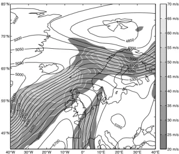
Fig. 2a.Synoptic chart for 00:00 UTC on 24 January 2003: Geopo-tential height at 500 hPa (contours) and wind speed (shaded).
2 Synoptic overview
The synoptic situation is described on the basis of analysis of surface and upper-air charts as given in the European Mete-orological Bulletin (http://dwd-shop.de/gb/0095.en.html) for the days 23 to 25 January 2003 and as shown by the European Centre for Medium Range Weather Forecasting (ECMWF) reanalysis for the same time-frame.
5750
5700 5600 5500
5400 5300 5200
5100 5050
5000
4950 4900
4800
4900
5000
5100
5200 5300
5400
5450
5400
40°W 30°W 20°W 10°W 0° 10°E 20°E 30°E 40°E
45°N 55°N 65°N 75°N 85°N
20 m/s 25 m/s 30 m/s 35 m/s 40 m/s 45 m/s 50 m/s 55 m/s 60 m/s 65 m/s 70 m/s
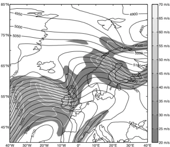
Fig. 2b.Synoptic chart for 06:00 UT on 25 January 2003: Geopo-tential height at 500 hPa (contours) and wind speed (shaded).
above 40 m/s around 300 hPa and 15 to 25 m/s between 850 and 500 hPa for the most part of the day.
3 Radiosonde observations
Altogether 8 GPS radiosondes were launched on 23 and 24 January 2003 as part of the MaCWAVE sounding rocket campaign (Goldberg et al., 2006). Here we use cleaned data sampled at 10 s (∼50 m) resolution. Profiles of wind speed and static stability, in terms of buoyancy frequency,ωB, are
shown by the blue lines in Fig. 4. Note that no wind mea-surements were available from the first sonde.
4 ESRAD observations
ESRAD is an interferometric VHF radar operating at 52 MHz. It is located at Esrange (Kiruna, Sweden, 67.9◦
N, 21.1◦
E) and has been operating essentially continuously since August 1996 (Chilson et al., 1999). The measurements used here are height profiles of signal strength, of vertical winds determined from the Doppler shift of the returned sig-nal, and of horizontal winds and r.m.s. velocity fluctuations determined by the full correlation (f.c.a.) technique (Briggs, 1984; Holdsworth et al., 2001; Holdsworth and Reid, 2004). The height resolution of the measurements on this occasion was 300 m, and each profile represents an average over 51 seconds, with measurements repeated each 2 min. The radar antenna (at the time of this case study) consisted of 140 yagi-antennas, arranged in a 12×12 square array (with 4 antennas missing in the centre). For echo power and vertical wind esti-mates, the whole antenna was used, corresponding to a beam
width of ∼6◦(full width, half maximum). For f.c.a. mea-surements, the whole array was used for transmission, but the array was divided into 6 rectangular sub-arrays, each of 4×6 antennas, for reception. Each f.c.a. measurement-point in a height profile corresponds to an average over a cylinder which is 300 m thick in the vertical direction and has a diam-eter which varies from∼180 m at 2000 m height to 900 m at 10 000 m height, vertically above the radar.
In principle, the height profile of radar echo power re-turned from the troposphere and lower stratosphere should depend on the distance from which the echo is returned, at-mospheric density, static stability, humidity gradients and the fine-scale structure of temperature and density fluctuations within the scattering volume (e.g. Gage, 1990). In practice, for vertically pointing radars operating around 50 MHz, the first three parameters have been found to dominate and echo power can be scaled to provide an estimate of static stability RB2=Fezexp(−z/H )Pr1/2 (1)
wherePr is radar echo power,zis height (also distance from
the radar),His the atmospheric scale height (so exp(−z/H ) gives the height variation of atmospheric density),RB=ωB,
the atmospheric buoyancy frequency, in the upper tropo-sphere and lower stratotropo-sphere (where humidity is negligible). Fe has been found to be independent of height and time at
least over heights from 5000–20 000 m in the upper tropo-sphere/lower stratosphere and over the several hours duration of the experiments so far reported (Hooper et al., 2004; Luce et al., 2007).
The constant of proportionalityFe can be found using a
single radiosonde and a check on the applicability of the equation is provided by comparing with further radiosondes. The radar-derivedRB are shown by the black lines in Fig. 4
(upper panel), where the first sonde has been used to deter-mineFe. The vertical resolution of the sonde measurements
is about 50 m, and the radar estimates have been averaged for 30 min following the sonde launch. The agreement between the radar-derivedRBand the sonde-derivedωBis good,
bear-ing in mind that the sondes do not sample exactly the same volume as the radar – by the time they reach the tropopause at∼8000 m they are typically∼40 km downwind. There is more detail in the vertical profiles measured by the sondes which is understandable since the radar averages over a nom-inal 300 m height interval (in practice a Gaussian-weighted height interval with a 300 m width at half power). In addition, the radar estimate does not capture the very low values of ωBsometimes found by the sondes in the upper troposphere
(14:00, 16:00, 19:00 and 22:00 UTC on 24 January), and on a few occasions in the lower troposphere (12 and 14:00 UTC on 23 January). The complete time-height series ofRB
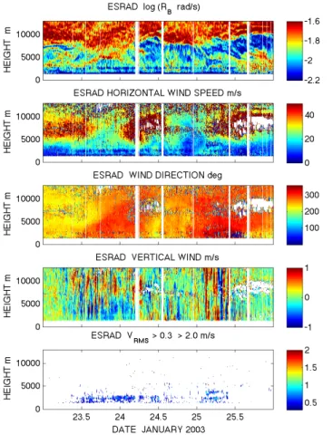
cal-culated from the radar echo power is shown in the top panel of Fig. 5a. The most conspicuous feature is the tropopause, marked by a rapid increase ofRBat heights varying between
S. Kirkwood et al.: Turbulence and mountain waves 3587
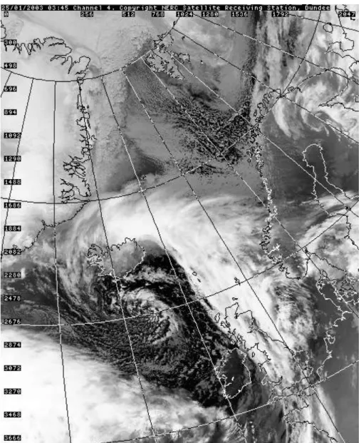
Fig. 3.Satellite cloud image at 03:45 UT on 25 January 2003 (NOAA, IR channel 4 from http://www.sat.dundee.ac.uk).
early on 24 January and early on 25 January. The high values ofRB throughout the upper troposphere (above 5000 m) on
the afternoon of 23 January, with no distinct tropopause (see also the first two radiosonde profiles in Fig. 4) , correspond to an equatorward extension of the deep depression centred further north, which is described in the synoptic overview.
The second and third panels (from the top) of Fig. 5a show the horizontal wind-speed and direction, determined by the f.c.a. technique. This technique assumes that a time-varying ensemble of scatterering structures (which may be anisotropic), are responsible for the radar echo. The signal scattered from these structures leads to a diffraction pattern on the ground, moving horizontally at twice the horizontal drift speed of the scatterers and changing over time. With an assumption that the temporal and spatial correlation func-tions of the diffraction pattern can be described by the same
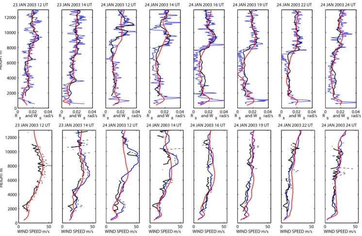
0 0.02 0.04 0
2000 4000 6000 8000 10000 12000
23 JAN 2003 12 UT
R
B and WB rad/s
HEIGHT m
0 0.02 0.04 23 JAN 2003 14 UT
R
B and WB rad/s
0 0.02 0.04 24 JAN 2003 12 UT
R
B and WB rad/s
0 0.02 0.04 24 JAN 2003 14 UT
R
B and WB rad/s
0 0.02 0.04 24 JAN 2003 16 UT
R
B and WB rad/s
0 0.02 0.04 24 JAN 2003 19 UT
R
B and WB rad/s
0 0.02 0.04 24 JAN 2003 22 UT
R
B and WB rad/s
0 0.02 0.04 24 JAN 2003 24 UT
R
B and WB rad/s
0 50
0 2000 4000 6000 8000 10000 12000
23 JAN 2003 12 UT
WIND SPEED m/s
HEIGHT m
0 50
23 JAN 2003 14 UT
WIND SPEED m/s
0 50
24 JAN 2003 12 UT
WIND SPEED m/s
0 50
24 JAN 2003 14 UT
WIND SPEED m/s
0 50
24 JAN 2003 16 UT
WIND SPEED m/s
0 50
24 JAN 2003 19 UT
WIND SPEED m/s
0 50
24 JAN 2003 22 UT
WIND SPEED m/s
0 50
24 JAN 2003 24 UT
WIND SPEED m/s
Fig. 4. Radiosonde measurements (blue), ESRAD radar measurements (black) and WRF model results for the ESRAD site (red). All
radiosondes were launched from the ESRAD site. ESRAD and WRF results are averaged for 30 min following the launch time. Top row shows buoyancy frequency, lower row wind speed. Solid black lines are f.c.a. true winds, dashed lines are apparent winds. See text for further details.
in the upper troposphere/lower stratosphere. In these cases the apparent wind speed is closer to that measured by the radiosonde. (There is no significant difference between the directions of the true, apparent and radiosonde winds.)
The fourth panel of Fig. 5a shows the vertical wind compo-nent measured by the radar. This is simply the mean Doppler shift of the echo, expressed in m/s, and with reversed sign so that positive values correspond to upward motion. This is determined using the whole antenna so it corresponds to a rather narrow radar beam (6◦
). In principle it is possible that these vertical winds might include a small component of horizontal wind, if scattering structures are systematically situated to one side of zenith. For example, a horizontal wind of 20 m/s would give an apparent vertical component of up to 1 m/s if a scatterer from a region 2◦off zenith dominates the returned signal. However, when we compare with the model results in the next section, we will see that there is no reason to believe that this is a significant effect. The vertical wind in Fig. 5a is characterised by alternating periods of strong (∼1 m/s) upward and downward motion, coherent over verti-cal distances of 5 km to at least 12 km. The amplitude of the
vertical winds is highest on the afternoon of the 23 January and the morning of 25 January, when the horizontal winds at low altitudes are from directions between west and north.
The fifth (bottom) panel of Fig. 5a shows when enhanced levels of turbulence are detected. This is based on the equiv-alent root mean square velocity spread, Vτ calculated from
the diffraction patterns intrinsic correlation time,τ, using the f.c.a. technique.
Vτ=λ(2ln2)1/2/4π τ (2)
whereλis the radar wavelength.
In the case that the scattering volume is filled with tur-bulent eddies, the latter will have random vertical veloc-ities. Averaging over the scattering volume and over the time of each measurement (51 s) will give Vτ =VRMS, the
S. Kirkwood et al.: Turbulence and mountain waves 3589
Fig. 5a. Measurements made by the ESRAD radar for 23, 24 and 25 January 2003. Gaps in the data due to interference, or low signal levels (signal-to-noise ratio<0.5) are shown in white. Top panel shows the logarithm of the radar estimate of buoyancy frequency,
RB. next two panels show the speed and direction of the horizon-tal wind (true wind from f.c.a. analysis). The direction from which the wind is blowing is given in degrees clockwise from north. The 4th panel shows the vertical wind from the Doppler shift of the radar echo (positive upwards). The lowest panel shows turbulent velocities (VRMS). Only values exceeding 0.3 m/s are plotted below
5500 m height, and values above 2 m/s above that height.
ESRAD, then gives a direct estimate of VRMS. There is no need for the kind of beam-width/wind-speed corrections which must be applied in the case of non-interferometric Doppler-beam-swinging radars which estimateVRMS from the spectral width of the echoes (see e.g. Cohn, 1995, for a discussion).
However, althoughVτ can be calculated for all heights and
times, it cannot always be assumed thatVτ=VRMS.
Short-lived quasi-specular reflections from sharp temperature gra-dients are also a source of low values ofVτ, particularly in the
upper troposphere and lower stratosphere (Kirkwood et al., 2010). Figure 6 shows height profiles of the median values of the radar signal strength and the diffraction-pattern cor-relation timeτ, for the three days of our case study. This shows two distinct regimes: high power (falling off with
Fig. 5b. Results from the WRF model, for 23, 24 and 25
Jan-uary 2003, innermost nested domain with 1 km grid spacing, for the location of the ESRAD radar. Top panel shows the logarithm of the buoyancy frequency,ωB. Next two panels show the speed and direction of the horizontal wind. The direction from which the wind is blowing is given in degrees clockwise from north. The 4th panel shows the vertical wind (positive upwards). The lowest panel shows the bulk Richardson number. See text for further details.
10!1 100 101 102
0 2000 4000 6000 8000 10000 12000
SIGNAL!TO!NOISE RATIO
HEIGHT m
0 1 2 3 4
0 2000 4000 6000 8000 10000 12000
LIFETIME s
distance from the radar) and long correlation times below 5500 m, low power and much shorter correlation times above 5500 m. It is well known that both turbulent eddies (vol-ume scatter) and quasi-specular reflection (fresnel scatter-ing) can contribute to the radar echoes from the lower atmo-sphere (e.g. Gage, 1990) and it is likely that the two distinct regimes in Fig. 6 correspond to these different mechanisms. We would not expect turbulence to be active at all heights and times, so we can use the median values as an indication of the diffraction-pattern correlation time due to non-turbulent processes, which correspond toVτ∼0.2 m/s in the lower tro-posphere where the median value ofτ∼2.5 s andVτ∼1 m/s at the upper heights where the median value ofτ∼0.5 s. We can be confident that the radar is detecting the signature of turbulence, and thatVτis a reasonable estimate ofVRMSonly
whenVτis significantly higher than these values. So the
low-est panel of Fig. 5a showsVRMS∼Vτ>0.3 m/s below 5000 m
height andVRMS∼Vτ>2 m/s above that height.
It is clear from Fig. 5a that high values ofVRMSprevail in the lower troposphere below about 4 km height, from midday on 23 January to midday on 25 January, and are most per-sistent during essentially the same intervals when mountain-wave signatures are strongest in the vertical wind. There are also scattered observations of highVRMSin the upper tropo-sphere on the morning of the 24 January and the afternoon of 25 January, but these are not as persistent as the turbulence at lower heights.
The first two radiosondes in Fig. 4 were launched at times when reasonably strong turbulence was detected by ESRAD, between 2000 and 3000 m height, at 12:00 and 14:00 UTC on 23 January . The next two sondes, at 12:00 and 14:00 UTC on 24 January coincide with enhanced turbulence seen by ESRAD in the upper troposphere. The sondes detected nar-row regions with very low values ofωB in the same height
regions as the radar turbulence observations. These would allow not only shear instability but, in some cases, convec-tive instability, consistent with the turbulence observed by the radar.
5 WRF-ARW model simulations
The WRF-ARW model, described by Skamarock et al. (2005, 2007) allows non-hydrostatic simulation of moun-tain waves based on high-resolution topography. Here we have used WRF version 2.1 with two-way nested domains, as shown in Fig. 1, with horizontal resolutions of 15 km (out-ermost domain), 3 km (intermediate domain) and 1 km (the innermost domain around the location of ESRAD), respec-tively. Results from the 1 km domain at the location of ES-RAD are illustrated in Fig. 5b. For the model runs, condi-tions at the outer boundary were provided by National Cen-ter for Environmental Protection (NCEP) final analyses at 1◦
, and 6 h resolution. For cloud microphysics, the 3-class simple scheme following Hong and Chen (2004) was used,
the 3 classes being vapour, cloud water/ice, rain/snow with ice or snow being assumed when the temperature is below freezing. For longwave radiation the RRTM look-up table scheme was used (Mlawer et al., 1997) and for shortwave radiation the scheme described by Dudhia (1989). No cu-mulus effects were included. The land surface is treated by a 5-layer surface thermal diffusion scheme (Skamarock et al., 2005, 2007). Runs were made with two different surface layer/boundary layer schemes (MM5-YSU and Eta-MYJ, Skamarock et al., 2005, 2007). Both schemes account for heat, moisture and momentum exchange with the sur-face, but use different models of turbulence in the bound-ary layer. No significant difference between the results us-ing the two schemes was found for the parameters studied in the present comparison. Runs were made using 50 hPa and 10 hPa top limits, and for several different vertical spacings of the model levels. No significant influence of the top height was found for the height region addressed here, i.e. between 0–13 000 m. The dependence of the results on the vertical resolution is discussed below. The results shown in Fig. 5b are for a model run using 66 model levels between the sur-face and 50 hPa with the spacing between model levels about 150 m up to 5000 m height, 350 m up to 10 000 m, and 500 m above there. Model runs were also made with 28 and 56 de-fault model levels, which have closer spacing in the boundary layer (up to∼1200 m) and about 700 m or 350 m spacing in the troposphere, respectively. Runs were further made both with, and without, the inner nested grids.
Figure 5b shows the model results in the inner domain (horizontal resolution 1 km), at the location of the ESRAD radar, at 5-minute resolution. The top 4 panels show buoy-ancy frequency, wind speed, wind direction, and vertical wind, respectively. Comparison with Fig. 5a shows that there is good agreement with the ESRAD measurements although there is more detail in the local observations on short time scales. This is unavoidable given the 6 h resolution of the input meteorological data for the model. Figure 4 provides a comparison of the WRF estimates (in red) ofωB and of
wind, with the radiosondes (blue) and with ESRAD (black). Here we can see that the model results, although agreeing in general tendencies, lack much of the detail of the real atmo-sphere. In particular, the radiosonde and radar measurements show much more structure in the profiles of wind speed, im-plying stronger wind-shears, compared to the model. Al-though the nominal vertical resolution of the model is 150 m, the model profiles are quite smooth even at this scale. This is likely the result of a lack of vertical resolution in the boundary conditions (i.e. the NCEP analyses). Further, the WRF winds underestimate upper-troposphere wind maxima (14:00 UTC on 23 January, 12:00 and 14:00 UTC on 24 Jan-uary). The WRF estimates ofωB show a very smooth
tran-sition in stability from the lower troposphere to the strato-sphere, in contrast to the sharp tropopause transition in the observations. The narrow regions where ωB is close to
S. Kirkwood et al.: Turbulence and mountain waves 3591 January, are not represented in the model. On the other hand,
a narrow zone withωBclose to zero is found in the model at
19:00 UTC on 24 January, but is not seen by the radiosonde (although the radiosonde seesωBclose to zero a little higher
up).
The 4th panel of Fig. 5b shows the vertical wind. The model reproduces both the amplitudes and the rapid changes in direction seen in the observations rather well. On 23 Jan-uary there is good agreement between model and observa-tions in vertical wavelength, amplitude and direction of the vertical wind. On 24 January the model amplitudes are some-what larger and the agreement is less good. On 25 January, the amplitudes agree well, but the vertical wavelength differs so that the signs of the perturbations in the model are op-posite in the upper troposphere, compared to the lower tro-posphere, whereas the observations show the same sign at all heights. The observed vertical winds are rather more variable in time than the modelled winds, which can give the impres-sion that the observed amplitudes are less. This comparison is considered in more detail below.
Figure 7 shows plan-views of the waves in the vertical wind, for 3 selected times, for the model level lying at 3000 m height above Esrange. The first example, at 00:00 UTC on 24 January, corresponds to surface wind from the southwest, the second to wind from the south-southwest, and the third to wind from the northwest. It is clear that the alignment of the wave fronts and the horizontal wavelength of the dominating waves varies with the wind direction. It is also clear that the amplitudes are highest when the wind is from the northwest, i.e. perpendicular to the mountain chain. Wavelengths vary between about 10 km, and about 20 km. In the first example, the longer wavelength dominates but a localised wave train with the smaller wavelength can be seen close to the ESRAD location. It is clear that the direction of the vertical wind at the ESRAD site will be very sensitive to the exact position of these waves. Given the temporal and spatial limitations of the meteorological data input to the model, it is not surpris-ing that there is no exact match in the timsurpris-ing of changes in vertical wind directions, between the model and ESRAD.
Additionally, any numerical model has inherent limita-tions. In this context it is of interest to consider whether the conditions are such as to lead to trapped waves which can be particularly difficult to model. Conditions for wave trap-ping are usually estimated using the Scorer parameter,l2=
ω2B/U2−(δ2U/δz2)/U, whereUis the horizontal wind, and the equation refers to conditions upstream of the mountains. When this parameter decreases substantially with increasing height, waves with wavenumber> lat the upper heights, will be trapped below. For our study period,lis relatively high in the lower troposphere but decreases in the upper troposphere more or less at the times and heights corresponding to the wind jets in Fig. 5. At these times, waves with horizontal wavelength less than∼20 km will tend to be trapped below the wind jets and accurate modelling may be difficult. At other times, specifically 12:00–20:00 UT on 23 January and
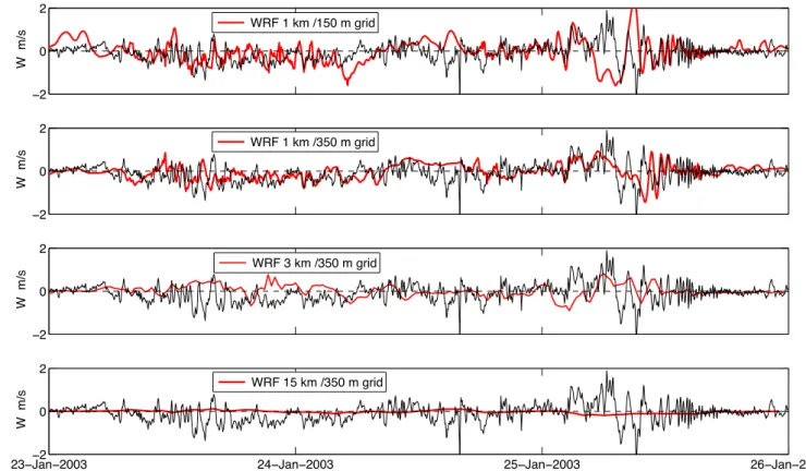
!2 0 2
W m/s
WRF 1 km /150 m grid
!2 0 2
W m/s
WRF 1 km /350 m grid
!2 0 2
W m/s
WRF 3 km /350 m grid
23!Jan!2003!2 24!Jan!2003 25!Jan!2003 26!Jan!2003
0 2
W m/s
WRF 15 km /350 m grid
Fig. 8.Comparison between vertical wind velocities measured by ESRAD and WRF model results using different horizontal (1, 3 or 15 km) and vertical (150 or 350 m) resolutions. Measurements and model results at 3000 m height.
12:00–20:00 UT on 24 January, the Scorer parameter varies little with height and waves should be free to propagate up-wards.
Figure 8 illustrates the sensitivity of the vertical wind to model parameters. Model runs with only the coarse-resolution, 15 km, grid give vertical wind perturbations an order of magnitude less than those observed by the radar. Us-ing the 3 km grid, the amplitudes of the vertical wind pertur-bations approach those observed, but the variability in time is much less, and there is rarely agreement in the sign. With the 1 km grid (either 350 m or 150 m vertical resolution) both the amplitude and the temporal variability in the vertical wind are reasonably well represented by the model. Over many intervals, there is also agreement in sign. The sensitivity to the horizontal resolution applies irrespective of height reso-lution, or of the model top-height used, although the exact details of the temporal variability are closest to the obser-vations when the highest vertical resolution (150 m) is used. We can also note that the agreement between the model and the measurements is not particularly better or worse during the periods when there should be no wave trapping (12:00– 20:00 UTC on 23 January and 12:00–20:00 UTC on 24 Jan-uary) than at other times.
The lowest panel of Fig. 5b shows the bulk Richardson number,Ri. Values less than 1 are generally considered
nec-essary to sustain wind-shear driven turbulence, less than 0.25
to initiate shear-driven turbulence. The model predicts such conditions in the boundary layer, below∼1200 m height, al-most all of the time. However, ESRAD is not able to make measurements at such low heights. Short periods withRi<1
are also predicted in the lower troposphere on the afternoon of 23 January, the afternoon of 24 January and the morning of 25 January. Values approaching this threshold are predicted in the upper troposphere on the afternoon of 25 January. The model also predicts a very short period of convective insta-bility (Ri<0) at about 18:00 UTC on 24 January (at 3000–
5000 m height). Clearly there is only a loose correlation be-tween the model and the radar observations concerning the occurrence of turbulence.
Figure 9 illustrates the sensitivity of the model results for Ri to the model parameters and compares in more detail
with the ESRAD observations. The model predictions of re-gions of lower-tropospheric turbulence (above the boundary layer), are not particularly sensitive to the horizontal reso-lution but are very sensitive to the height resoreso-lution used. Intervals when turbulence could be sustained (Ri<1) and of
shear-driven instability (Ri<0.25) are occasionally predicted
by the model, for any horizontal resolutions (15, 3 or 1 km, only 15 and 1 km are shown in Fig. 9) so long as the height resolution is 350 m or less. The depth of the minima inRi
S. Kirkwood et al.: Turbulence and mountain waves 3593
0 0.5 1
V
R
M
S
m/s ESRAD turbulence
23!Jan!2003 24!Jan!2003 25!Jan!2003 26!Jan!2003
0 2 4 6 >
RICHARDSON NUMBER
WRF 1 km / 150 m
WRF 15 km /150 m
WRF 15 km /350 m
WRF 15 km /700 m
Fig. 9. Comparison between turbulent velocities measured by ESRAD and WRF model estimates of the bulk Richardson number using
different horizontal (1 or 15 km) and vertical (150, 350 or 700 m) resolutions. Measurements show the meanVRMSbetween 2000 and
5000 m heights, model results the minimum Richardson number between the same heights.
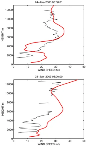
0 10 20 30 40 50
0 2000 4000 6000 8000 10000 12000
WIND S/EED 12s
HEIGHT 1
24!78n!2003 00:00:01
0 10 20 30 40 50
0 2000 4000 6000 8000 10000 12000
WIND S/EED 12s
HEIGHT 1
25!78n!2003 06:00:00
Fig. 10.Comparison of wind profiles between WRF (red) and ES-RAD (black). At 00:00 UTC on 24 January and at 06:00 UTC on 25 January.
instability,Ri<0, are seen only when 1 km horizontal
resolu-tion is used for the model. The intervals of lowRi, at around
00:00 UTC on 24 January, 18:00–19:00 UTC on 24 January, to a lesser extent at 04:00–06:00 UTC on 25 January, are much shorter than the duration of theVRMSenhancement ob-served by ESRAD. Also, the peaks inVRMSdo not appear at exactly the times of lowestRi.
The situation at 19:00 UTC on 24 January, where the model predicts convective instability at about 5000 m height, can be seen in more detail in Fig. 4. It can be seen that the ra-diosonde does not detect such low buoyancy frequency as the model predicts, in agreement with the lack of turbulence de-tected by the radar at that height. Figure 10 examines in more detail the differences between the model results and ESRAD observations at 2 further times. At 00:00 UTC on 24 January, the model predicts a wind minimum at 4000 m height, with strong shears above and below, which lead to low values of Ri. There is no wind minimum in the ESRAD observations
at this time and no turbulence at 4000 m height. The opposite applies at 06:00 UTC on 25 January, when ESRAD detects a wind minimum, shears and turbulence, while the model does not predict this. Clearly small differences like this can ex-plain a lack of exact match between model predictions for lowRi and observed turbulence.
65 66 67 68 69 70 71 72 0
2000 4000 6000 8000 10000 12000 14000
LATITUDE
HEIGHT
WRF WB N−S section ESRAD longitude 2003−01−24 00:00:00
10 10
20
20
20
20 20
20
20 30
30
30
30
30 30
30 0.005
0.01 0.015 0.02
65 66 67 68 69 70 71 72
0 2000 4000 6000 8000 10000 12000 14000
LATITUDE
HEIGHT
WRF W
B N−S section ESRAD longitude 2003−01−25 06:00:00
10
1020 20 10
20
20
30 30
30
30
40
40
40
0.005 0.01 0.015 0.02
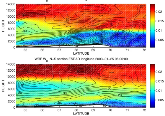
Fig. 11.Latitude-height cross sections of buoyancy frequency (colour scale, units s−1) and wind speed (contours, units m/s) from an extended
outermost model domain (15 km horizontal grid). The cross sections are at the ESRAD longitude.
overlies a shallower airmass from the north, with relatively low static stability. Note that the low-stability airmass is much deeper on 24 January (5000 m at the ESRAD latitude of 68◦
) than on 25 January (2000 m at ESRAD). The wind speed increases sharply in height at about the location of the sloping boundary between the two air masses. (Both exam-ples can be recognised as tropopause folds as described in Rao and Kirkwood, 2005, although this is clearest for the example for 24 January). A combination of high windshear and low stability favours turbulence. Above the lee of the mountains (68◦–69◦N) both the static stability and the wind speed show wave-like variations in height. These are sig-natures of long-wavelength inertial gravity waves which can lead to combinations of low stability and high wind shear at slightly different latitudes and heights depending on the exact location of these waves. Inertial gravity waves for this time period, with horizontal wavelengths of 100 s of km, and ver-tical wavelengths of a few km, have been modelled by Serafi-movich et al. (2006), who found that both orographic effects and the upper-troposphere wind jet contributed to generating the waves. In reality, further perturbations will be added to those inertial waves i.e. from the waves with 10–20 km hori-zontal wavelength, which are not present in the model results at 15 km horizontal resolution. These high-amplitude small-scale waves can result in localised reduction of the static sta-bility in parts of the wave field. This is illustrated by Fig. 12, which shows E–W cross-sections for the high-resolution
do-main, through ESRAD. Thin wave-induced layers of convec-tive instability, i.e.ωB<0 (enclosed by the white contour),
can be seen in parts of the wave field.
Figure 13 considers average occurrence rates for lence (from ESRAD) and for conditions supporting turbu-lence (from WRF at the ESRAD location). Figure 13 shows averages over the whole 3-day case study period. Enhanced turbulence levels are rather more common than intervals of Ri<1, with turbulence occurrence rates closer to those
for Ri<2. In the lower troposphere, the height profiles of
VRMS>0.3 m/s and of Ri<2 are similar. Peak occurrence
rates of both conditions have values 0.4–0.6 between 2000 m and 3000 m heights and fall off in similar ways towards the upper troposphere. In the upper troposphere the occurrence rates of bothVRMS>2 m/s and ofRi<2 are very low.
Consid-ering that thin layers with lowωB, or higher wind shear, are
more common in the radiosonde profiles than in the model, it seems likely that regions of lowRi in the lower troposphere
are simply not resolved by the model resolution, so their oc-currence rate is underestimated.
S. Kirkwood et al.: Turbulence and mountain waves 3595
Fig. 12. Longitude-height cross sections of buoyancy frequency (colour scale, units s−1) and potential temperature (black contours,
units K). White contours enclose regions of convective instability, i.e. buoyancy frequency<0. From the innermost model domain (1 km horizontal grid) at the ESRAD latitude.
corresponding reasonably well to regions where the WRF model simulated a lowering of Richardson number to values between 0.5 and 2.
6 Discussion
The model results tell us that the turbulence we observe in the lower troposphere occurs in the same conditions as mountain-waves. However, while the dominant mountain waves in the model, with 10–20 km horizontal wavelength are most sensitive to the horizontal resolution used, the con-ditions for turbulence are most sensitive to the vertical res-olution. This suggests that the mountain waves are not the direct cause of the turbulence at the radar site. This is fur-ther supported by Fig. 14, which shows occurrence rates for various conditions over the whole area covered by the in-termediate model domain. The region whereRi<2 is
com-mon, i.e. likely turbulence, is very different from the region where high vertical winds are common, i.e. high-amplitude mountain waves. As we have seen in the sections above, in
0 0.2 0.4 0.6 0.8 1
0 2000 4000 6000 8000 10000 12000
OCCURRENCE RATE
HEIGHT m
ESRAD 23−25 JANUARY 2003
V
RMS >0.6
V
RMS >0.3
V
RMS >2.0
0 0.2 0.4 0.6 0.8 1
0 2000 4000 6000 8000 10000 12000
OCCURRENCE RATE
HEIGHT m
WRF at Esrange location 23−25 JANUARY 2003
Ri < 0 Ri < 0.25 Ri < 1 Ri < 2
Fig. 13. Occurrence rates of turbulence observed by ESRAD, and low Richardson numbers predicted by WRF for the ESRAD loca-tion, for the whole period 23rd–25th January, 2003. WRF results based on 1 km/150 m grid resolution.
the lower troposphere, turbulence is primarily due to strong wind shears, localised in height, but extended horizontally over large parts of the model domain. These are associated with wind shear at upper-level fronts which separate rela-tively stable air from the south from relarela-tively unstable air from the north. Although this is the main underlying cause of conditions supporting turbulence, perturbations due to the mountain waves can act to further decreaseRi, particularly
by reducingωBin some parts of the waves, as can be seen in
Fig. 12.
Fig. 14.Plan view of the occurrence rates ofωB<0, vertical shear in horizontal wind>0.001s−1, Richardson number<2, and vertical wind
>1 m/s. Occurrence rates give the average for the period 23–25 January 2003 and for the height interval 2000–5000 m and are plotted first based on WRF simulations for an extended domain with 3 km horizontal and 150 m vertical resolution. Results for the 1 km grid are then superposed.
is a possible source of turbulence which is likely not cap-tured accurately by our WRF simulations. Records of the cloud cover during our case study exist in the form of all-sky photographs during the night hours, from a camera lo-cated 20 km east of the radar site which monitors the aurora (http://www.irf.se/allsky/), and in the records of lidar obser-vations from the same site as the radar (K. H. Fricke, personal communication, 2003; Blum et al., 2006). Both of these sources showed that there were clear skies during most of the time, between 19:00–04:00 UTC on the night 23/24 January and between 23:00–06:00 UTC on 24/25 January. The turbu-lent layers in the lower troposphere were seen by the radar throughout those periods, so the turbulence cannot have been due to cloud-induced effects.
The model itself does not completely explain the ob-served occurrence of turbulence if we consider that the bulk Richardson number should be less than 1 to support tur-bulence. On a case-by-case basis there is poor agreement
between model predictions of low Richardson number and observation of turbulence by the radar. However, there is reasonable agreement in the height profiles of overall occur-rence rates of low Richardson number (Ri<2) and observed
turbulence. The onset of turbulence around midday on 23 January and its continuation for a further 24 h coincide with the onset and persistence of conditions of low Richardson number in the model. Subsequently, however, the agreement in time is poor.
S. Kirkwood et al.: Turbulence and mountain waves 3597
0 0.1 0.2 0.3 0.4 0
2000 4000 6000 8000 10000 12000
OCCURRENCE RATE
HEIGHT
WRF 1km GRID 23−25 JANUARY 2003
0 0.2 0.4 0.6 0.8 1 0
2000 4000 6000 8000 10000 12000
OCCURRENCE RATE
HEIGHT
WRF 1km GRID 23−25 JANUARY 2003
Ri
MIN<0
Ri<0 Ri<0.25 Ri<1 Ri<2
Fig. 15.Left-hand side : occurrence rates for low values of Richard-son number for the whole of the innermost model domain, and for the period from 00:00 UTC on 23 January to 24:00 UTC on 25 Jan-uary 2003. Right-hand side: the average (over latitude and time) of the occurrence rate of convective instability at any location along a latitude circle, within the innermost model domain. This represents the chance that an air-mass crossing the domain will encounter a region of convective instability somewhere along its path from west to east.
measured directly byVRMS2 ) is converted to vertical mixing or eddy diffusivity (which implies an increase in potential en-ergy). The physics of turbulent mixing in a stably-stratified atmosphere has been addressed by Weinstock (1978), leading to an expression for vertical eddy diffusivityK
K∼0.4VRMS2 /ωB (3)
(Note that the value of the numerical constant in this ex-pression varies between different derivations. The value here, 0.4, is among the highest found in the literature, while Kurosaki et al., 1996, for example, use one of the lowest val-ues, 0.1). The characteristic time for vertical mixing (for ex-ample the relaxation of the vertical gradient in ozone mixing ratio, assuming no new sources), is given by (e.g. Goody, 1995)
tK∼H2/K (4)
wheheH is the density scale height, which is ∼7 km. In terms of measuredVRMS, this gives
tK∼2.5ωBH2/VRMS2 (5)
Clearly, tK will be very sensitive to the buoyancy
fre-quencyωB. The mean value ofωBin the conditions ofRi<2
at the location of ESRAD (for the WRF results shown in Fig. 5b) is 10−2s−1. For the rather high value ofVRMS=1 m/s, this would lead totK∼14 days, which would imply a rather
slow rate of mixing. On the other hand,tKwill be reduced to
zero in conditions of convective instability (ωB≤0). The
the-oretical considerations of Weinstock (1978) do not really ap-ply in these conditions. However, 3-D turbulence simulations
of breaking waves (which is essentially the conditions which here would correspond toωBfalling to zero) have shown that
mixing is indeed very rapid, with time scale of the order of a buoyancy period (Fritts et al., 2003).
The possibility that air masses flowing across the moun-tains might encounter regions of convective instability, is very important for the possibility of rapid vertical mixing. Figure 15 shows the occurrence rate of low Richardson num-bers averaged over the whole inner model domain, and, on the right hand side, the chance that an air mass will en-counter convective instability. The domain-averaged occur-rence rates of low Richardson number are much like those for the ESRAD site alone (Fig. 13), however when consid-ered in terms of the chance of convective mixing anywhere along the path, the rates are much higher, 5–10%. Since the time spent by an air mass in crossing such a region (Fig. 12) will be of the order of a buoyancy period, the air within the layer affected can be completely mixed. Although mixing at any particular place and time is likely to be confined to a thin layer, the air column is likely to encounter further mix-ing layers at slightly different heights as it flows across the mountains.
As we have seen in the radiosonde comparison, the model seems to underestimate the occurrence of thin layers of very lowωB so that the 5–10% chance of convective mixing in
Fig. 15 may be an underestimate. However, the uncertainty in this is too large to allow us to make direct quantitative predictions of vertical mixing on the basis of the model re-sults alone. The radar measurements can be used to examine the occurrence rates of various levels of turbulence(VRMS2 ) but uncertain assumptions on the corresponding values ofωB
would be needed to estimatetK.
7 Conclusions
Radar observations over a longer time can reasonably be used to make a qualitative assessment of the occurrence of turbulent mixing in the lower troposphere, its variations over time on different scales (hours to seasonal), over height, and its relation both to synoptic systems and to mountain waves. There is a large uncertainty, and possibly a large scatter, in the buoyancy frequency within the narrow layers where tur-bulent mixing most likely takes place. This makes it difficult to make quantitative estimates of the overall time scale of vertical mixing in the air-flow over the region, using only the radar observations or the WRF model results.
Comparison of height profiles of a suitable tracer, such as ozone in wintertime, at different points along the path of air-flow across the mountains, would be a possible method to examine this problem further.
Acknowledgements. The ESRAD radar is jointly owned and
operated by Swedish Institute of Space Physics and Swedish Space Corporation. This research has been made possible by grants from Swedish Research Council, Swedish Development Agency and the Kempe foundation. WRF was developed at the National Center for Atmospheric Research (NCAR) which is operated by the University Corporation for Atmospheric Research (UCAR). Cloud images (from NOAA GOES satellite) are archived and provided by the NERC Dundee satellite Center. Meteorological data from the NCEP Global Forecasting system data were provided by the Data Support Section of the Computational and Information Systems Laboratory at the National Center for Atmospheric Research. NCAR is supported by grants from the National Science Foundation. We thank R. Goldberg and F. Schmidlin, NASA, for providing radiosonde data which were part of the MaCWAVE sounding rocket campaign.
Edited by: G. Vaughan
References
Blum, U., Baumgarten, G., Schoech, A., Kirkwood, S., Naujokat, B., and Fricke, K. H.: The atmospheric background situation in northern Scandinavia during January/February 2003 in the con-text of the MaCWAVE campaign, Ann. Geophys., 24, 1189– 1197, 2006, http://www.ann-geophys.net/24/1189/2006/. Briggs, B. H.: The analysis of spaced sensor records by correlation
techniques, in: Handbook for MAP, 13, 166–186, Univ. of Ill., Urbana, 1984.
Chilson, P., Kirkwood, S., and Nilsson, A.: The Esrange MST radar: A brief introduction and procedure for range validation using bal-loons, Radio Sci., 34, 427–436, 1999.
Cohn, A.: radar measurements of turbulent eddy dissipation rate in the troposphere : a comparison of techniques, J. Atmos. Ocean. Tech., 12, 85–95, 1995.
Dibb, J., Talbot, R., Scheuer, E., Seid, G., DeBell, L., Lefer, B., and Ridley, B.: Stratospheric influence on the northern North American free troposphere during TOPSE: 7Be as a stratospheric tracer, J. Geophys. Res., 108, 8863, doi:10.1029/2001JD001347, 2003.
D¨ornbrack, A.: Turbulent mixing by breaking gravity waves, J. Fluid Mech., 375, 113–141, 1998.
D¨ornbrack, A., Birner, T., Fix, A., Flentje, H., Meister, A., Schmid, H., Bromwell, E., and Mahoney, M.: Evidence for intertia grav-ity waves forming polar stratospheric clouds over Scandinavia,, J. Geophys. Res., 107, 8287, doi:10.1029/2001JD000452, 2002. Doyle, J. D. and Durran, D. R.: Recent developments in the the-ory of atmospheric rotors, B. Am. Meteorol. Soc., 85, 337–342, doi:10.1175/BAMS-85-3-337, 2004.
Doyle, J. D. and Durran, D. R.:The dynamics of mountain-wave induced rotors, J. Atmos. Sci., 59, 186–201, 2002.
Doyle, J., Shapiro, M., Jiang, Q., and Bartels, D.: Large-amplitude mountain wave breaking over Greenland, J. Atmos. Sci., 62, 3106–3126, 2005.
Dudhia, J.: Numerical study of convection observed during the winter monsoon experiment using a mesoscale two-dimensional model, J. Atmos. Sci., 46, 3077–3107, 1989.
Fritts, D. C., Bizon, C., Werne, J. A., and Meyer, C. K.: Lay-ering accompanying turbulence generation due to shear insta-bility and gravity wave breaking, J. Geophys. Res, 108, 8452, doi:10.1029/2002JD002406, 2003.
Fukao, S., Yamanaka, M. D., Ao, N., Hocking, W. K., Sato, T., Yamamoto, M., Nakamura, T., Tsuda, T., and Kato, S.: Seasonal variability of vertical eddy diffusivity in the middle atmosphere 1. Three-year observations by the middle and upper atmosphere radar, J. Geophys. Res., 99, 18973–18987, 1994.
Gage, K.: Radar observations of the free atmosphere : structure and dynamics, in: Radar in Meteorology, edited by: Atlas, D., American Meteorological Society, Boston, USA, 534–565, 1990. Goldberg, R. A., Fritts, D. C., Schmidlin, F. J., Williams, B. P., Croskey, C. L., Mitchell, J. D., Friedrich, M., Russell III, J. M., Blum, U., and Fricke, K. H.: The MaCWAVE program to study gravity wave influences on the polar mesosphere, Ann. Geophys., 24, 1159–1173, 2006,
http://www.ann-geophys.net/24/1159/2006/.
Goody, R.: Principles of atmospheric chemistry and physics, Ox-ford University Press, New York, USA, 264–266, 1995. Hoffmann, P., Serafimovich, A., Peters, D., Dalin, P., Goldberg, R.,
and Latteck, R.: Inertia gravity waves in the upper troposphere during the MaCWAVE winter campaign – Part I: Observations with collocated radars, Ann. Geophys., 24, 2851–2862, 2006, http://www.ann-geophys.net/24/2851/2006/.
Holdsworth, D. A., Vincent, R. A., and Reid, I. M.: Mesospheric turbulent velocity estimation using the Buckland Park MF radar, Ann. Geophys., 19, 1007–1017, 2001,
http://www.ann-geophys.net/19/1007/2001/.
Holdsworth, D. A. and Reid, I. M.: Comparisons of full correlation analysis (FCA) and imaging Doppler interferometry (IDI) winds using the Buckland Park MF radar, Ann. Geophys., 22, 3829– 3842, 2004, http://www.ann-geophys.net/22/3829/2004/. Hong, S.-Y., J. D. and Chen, S.-H.: A revised approach to ice
mi-crophysical processes for the bulk parameterization of clouds and precipitation, Mon. Weather Rev., 132, 103–120, 2004. Hooper, D. A., Arvelius, J., and Stebel, K.: Retrieval of atmospheric
static stability from MST radar return signal power, Ann. Geo-phys., 22, 3781–3788, 2004,
http://www.ann-geophys.net/22/3781/2004/.
S. Kirkwood et al.: Turbulence and mountain waves 3599
doi:10.1029/2002JD002639, 2003.
Kurosaki, S., Yamanaka, M. D., Hashiguchi, H., Sato, T., and Fukao, S.: Vertical eddy diffusivity in the lower and middle at-mosphere: A climatology based on the MU radar observations during 1986–1992, 58, 727–734, 1996.
Kirkwood, S., Belova, E., Satheesan, K., Rao, T. N., Satheesh, K. S. and Prasad, T. R.: Fresnel scatter revisited - Comparison of radar and radiosonde data from the Arctic, the tropics and Antarctica, Ann. Geophys., submitted, 2010.
Larsson, L.: Observations of lee wave clouds in the J¨amtland Moun-tains, Sweden, Tellus, 6, 124–138, 1954.
Luce, H., Hassenpflug, G., Yamamoto, M., and Fukao, S.: Compar-isons of refractive index gradient and stability profiles measured by balloons and the MU radar at a high vertical resolution in the lower stratosphere, Ann. Geophys., 25, 47–57, 2007,
http://www.ann-geophys.net/25/47/2007/.
Maturilli, M. and D¨ornbrack, A.: Polar stratospheric ice cloud above Spitsbergen, J. Geophys. Res., 111, doi:10.1029/2005JD006967, 2006.
Mlawer, E., Taubman, S., Brown, P., Iacono, M., and Clough, S.: Radiative transfer for inhomogeneous atmospheres: RRTM, a validated correlated-k model for the longwave, J. Geophys. Res., 102, 16663–16682, 1997.
Nastrom, G. D., Gage, K. S., and Ecklund, W. L.: Variability of Turbulence, 4–20 km, in Colorado and Alaska From MST Radar Observations, J. Geophys. Res., 91, 6722–6734, 1986.
Nastrom, G. and Eaton, F.: Turbulence eddy dissipation rates from radar observations at 5–20 km at White Sands Missile Range, New Mexico, 102, 19495–19505, 1997.
Nastrom, G. D. and Eaton, F. D.: Seasonal variability of turbulence parameters at 2 to 21 km from MST radar measurements at Van-denberg Air Force Base, California, 110, 19495–19505, 2005. Pluogonven, R., Hertzog, A., and Teitelbaum, H.: Observations
and simulations of a large-amplitude mountain wave breaking over the Antarctic Peninsula, J. Geophys. Res., 113, D16113, doi:10.1029/2007JD009739, 2008.
Rao, D. N., Rao, T. N., Venkataratnam, M., Thulasiraman, S., Rao, S. V. B., Srinivasulu, P., and Rao, P. B.: Diurnal and seasonal variability of turbulence parameters observed with In-dian mesosphere-stratosphere-troposphere radar, Radio Sci., 36, 1439–1457, 2001.
Rao, T. and Kirkwood, S.: Characteristics of tropopause folds over Arctic latitudes, J. Geophys. Res., 110, D18102, doi:10.1029/2004JD005374, 2005.
Rao, T. N., Kirkwood, S., Arvelius, J., von der Gathen, P., and Kivi, R.: Climatology of UTLS ozone and the ratio of ozone and potential vorticity over northern Europe, J. Geophys. Res., 108, 4703–4711, doi:10.1029/2003JD003860, 2003.
Rao, T. N., Arvelius, J., and Kirkwood, S.: Climatology of tropopause folds over a European Arctic station (Esrange), J. Geophys. Res., 113, D00B03, doi:10.1029/2007JD009638, 2008.
R´echou, A., Barabash, V., Chilson, P., Kirkwood, S., Savitskaya, T., and Stebel, K.: Mountain wave motions determined by the Esrange MST radar, Ann. Geophys., 17, 957–970, 1999, http://www.ann-geophys.net/17/957/1999/.
Serafimovich, A., Z¨ulicke, Ch., Hoffmann, P., Peters, D., Dalin, P., and Singer, W.: Inertia gravity waves in the upper troposphere during the MaCWAVE winter campaign – Part II: Radar investi-gations and modelling studies, Ann. Geophys., 24, 2863–2875, 2006, http://www.ann-geophys.net/24/2863/2006/.
Skamarock, W., Klemp, J., Dudhia, J., Gill, D., Barker, D., Wang, W., and Powers, J.: A description of the Advanced research WRF version 2,, NCAR Tech. Note NACR/TN-468+STR, National center for Atmospheric Research, Boulder, Colorado, 2005, re-vised, 2007.
Sprenger, M. and Wernli, H.: A northern hemisphere cli-matology of cross-tropopause exchange for the ERA15 time period (1979–1993), J. Geophys. Res., 108, 8251, doi:10.1029/2002JD002636., 2003.
Stohl, A.: Characteristics of atmospheric transport into the Arctic troposphere, J. Geophys. Res., 111, D11306, doi:10.1029/2005JD006888, 2006.
Stohl, A., Forster, C., Frank, A., Seibert, P., and Wotawa, G.: Tech-nical note: The Lagrangian particle dispersion model FLEX-PART version 6.2, Atmos. Chem. Phys., 5, 2461–2474, 2005, http://www.atmos-chem-phys.net/5/2461/2005/.
Tarasova, O. A., Brenninkmeijer, C. A. M., Jckel, P., Zvyagintsev, A. M., and Kuznetsov, G. I.: A climatology of surface ozone in the extra tropics: cluster analysis of observations and model results, Atmos. Chem. Phys., 7, 6099–6117, 2007,
http://www.atmos-chem-phys.net/7/6099/2007/.
Valkonen, T., Vihma, T., Kirkwood, S., and Johansson, M.: Fine-scale model simulation of gravity waves gener-ated by Basen nunatak in Antarctica, Tellus, 62A, 319–332, doi:10.1111/j.1600-0870.2010.00443.x, 2010.
Vihma, T., L¨upkes, C., Hartmann, J., and Savij¨arvi, H.: Observa-tions and modelling of cold-air advection over Arctic sea-ice, Bound.-Lay. Meteorol., 117, 275–300, doi:10.1007/s10546-004-6005-0, 2005.
Vosper, S. B. and Worthington, R. M.: VHF radar measurements and model simulations of mountain waves over Wales, Q. J. Roy. Meteor. Soc., 128, 185–204, doi:10.1256/00359000260498851, 2002.
Wang, L., Fritts, D. C., Williams, B. P., Goldberg, R. A., Schmidlin, F. J., and Blum, U.: Gravity waves in the middle atmosphere during the MaCWAVE winter campaign: evidence of mountain wave critical level encounters, Ann. Geophys., 24, 1209–1226, 2006, http://www.ann-geophys.net/24/1209/2006/.
Weinstock, J.: Vertical turbulent diffusion in a stably stratified fluid, J. Atmos. Sci., 35, 1022–1027, 1978.