A sensorless control for a variable speed wind turbine operating at partial load

A sensorless control for a variable speed wind turbine operating at partial load

Ronilson Rocha

School of Mines, Department of Engineering of Control and Automation, Federal University of Ouro Preto, Campus Morro do Cruzeiro, 35400-000 Ouro Preto, MG, Brazil

a r t i c l e

i n f o

Article history: Received 3 August 2009 Accepted 4 June 2010 Available online 29 June 2010

Keywords: Wind energy

Stall regulated wind turbine Sensorless control LQG/LTR methodology

a b s t r a c t

This paper presents a sensorless control for a variable speed wind turbine (WT) operating at partial load in order to eliminate the direct measurement of the wind speed. In this proposal, the estimated aero-dynamic torque is used to determine the optimal reference of the speed control for maximum energy conversion. The maximization of the efficiency on energy conversion and the minimization of detri-mental dynamical loads are control trade-offs considered in the design of an optimal discrete-time feedback LQG/LTR controller for the Wind Energy Conversion System (WECS), which is based on the optimization of a quadratic cost function. The performance of the proposed control when the WT is submitted to a gust or step variation on wind speed is evaluated from computational simulations. It is also presented some proposals for sensorless control of the electrical generator.

Ó_{2010 Elsevier Ltd. All rights reserved.}

1. Introduction

Due to signi_ficant cost reductions, improved ef_ficiency and the increased useful life provided by the technological development of wind energy conversion systems (WECS), wind power is considered one of the most attractive solutions to energy prob-lems. The basic con_figuration of a WECS is shown inFig. 1. It is composed by a wind turbine (WT) coupled to an electrical generator, directly or through gear-box. In spite of its simplicity, the WECS represents an interesting problem in viewpoint of the control theory, since it is a nonlinear system, subjected to cyclical disturbances caused by operational phenomena, and highly dependent of a stochastic variable characterized by sudden vari-ations. Thus, the quality of a WECS controller is determined by its capacity to deal with model uncertainties, exogenous stochastic signals, and periodic disturbances.

Although classical methods are traditionally utilized in WECS control, these solutions are not completely adequate since the resulting controllers do not provide sufficient damping to system and the necessary robustness to uncertainties, such as parameter variations, nonlinear behavior, etc[1e5]. In this context, the linear quadratic gaussian controller with loop transfer recovery (LQG/LTR) consists in an interesting alternative for WECS, since it combines the necessary characteristics to assure the stability margin, disturbance attenuation and a reasonable robustness to model uncertainties[6,7]. Furthermore, the control trade-offs for a WECS can be easily translated into a quadratic cost function[3,8], which is inherent to design of an optimal linear feedback LQG/LTR controller.

The information related to wind speed is essential for the control of a WECS. However, the use of anemometers to measure the wind speed can represent a serious obstacle to implement a robust control structure for a WECS[9,10]:

The possible contamination of the reference signal by the wind

fluctuation, which can be solved _filtering the measurement signal;

The wind speed can not be measured exactly in the WT rotor, which dif_ficulties the exact evaluation of the available power for energy conversion;

The installation of the anemometer can reduce the reliability of the measure of wind speed due to aerodynamic interference, shadowing effects, turbulences, etc.

Another fundamental information for WECS control is the position or the rotation of mechanical shaft, which can be measured using tachometers, encoders and resolvers. However, the use of these transducers can also introduce others problems:

These transducers are often one of the most expensive and fragile components in a WECS, principally for small and medium power systems;

The space limitations and difficult access to the mechanical shaft can implicate in restrictions to use of a speed sensor; The additional wires for electrical connections of a speed

sensor can increase the vulnerability of the system to electro-magnetic interferences (EMI);

Problems related to assembling and maintenance. E-mail address:rocha@em.ufop.br.

Contents lists available atScienceDirect

Renewable Energy

j o u r n a l h o m e p a g e : w w w . e l s e v i e r . c o m / l o c a t e / r e n e n e

0960-1481/$esee front matterÓ2010 Elsevier Ltd. All rights reserved. doi:10.1016/j.renene.2010.06.008

Thus, the direct measurement of the wind speed, position and rotation of the mechanical shaft can represent a great obstacle to the implementation of a more ef_ficient, robust and cheap WECS, since the related sensors can be extremely expensive and introduce several uncertainties in the system. In this context, the elimination of the direct measurements of the mechanical variables in the control system consists in a very attractive perspective in the technical and economical viewpoints for WECS design, principally for small and medium systems.

This paper presents a sensorless control for a variable speed WT operating at partial load, aiming the elimination of the direct measurement of the wind speed. In this proposal, the estimated aerodynamic torque is used to determine the optimal reference of the speed control for maximum energy conversion. The maximi-zation of the efficiency on energy conversion and the minimization of detrimental dynamical loads are control trade-offs considered in the design of an optimal discrete-time feedback LQG/LTR controller for the Wind Energy Conversion System (WECS), which is based on the optimization of a quadratic cost function. The performance of the proposed control when the WT is submitted to a gust or step variation on wind speed is evaluated from computational simula-tions. It is also presented some proposals for sensorless control of the electrical generator.

2. Nonlinear WECS model

The WECS dynamics are presented inFig. 2. For the computational simulation of the system, it is necessary a complex and consistent nonlinear WT model that consider several operational phenomena, such as losses, wind shear, ripple torque, and turbulence. Assuming

a single dimensional random process, a nonlinear dynamic model for WT system can be divided in four distinct subsystems[11]: wind, aerodynamics, driven train and electrical generator. In the approach adopted in this paper, the structural dynamics are neglected and considered as model uncertainties.

2.1. Wind

An adequate model of the wind is necessary to predict the dynamics of a WECS. Although the wind is a multidimensional stochastic process, which depends on the time and spatial coordi-nates, a two dimensional model is generally enough to describe adequately this phenomenon [11]. The wind speed VH at the reference heightHcan be given by[12,13]:

VH ¼ Vþ

D

VþVGþVR (1)

whereVis the effective average of the wind speed over the WT rotor and

D

Vis the windfluctuation given by:

D

_{V ¼ 2}X N

i¼1

½Svð

u

_iÞ

D

u

Š

1 2_cosð

_u

itþ

F

iÞ (2)

where

u

i¼ ði ð1=2ÞÞ

D

u

,

F

iis an independent random variable with uniform density in the interval of 0e2

p

andSv(

u

i) is the power spectral density, given by[11]:

Svð

u

_iÞ ¼

2KNF2j

u

ij

p

2h_1þFui

mp

2i4 3

(3)

Fig. 1.Basic WECS configuration.

whereKNis the superficial drag coefficient,Fis the turbulence scale, and

m

is the average of the wind speed in the reference height. For good results, it is suggestedN¼50 and

D

u

between 0.5 and 2.0 rad/s[14]. Since the wind speed depends of the height due to“wind shear”, an approach to compute the wind speed at a specific height his given by[11,15,16]:

Vh ¼ VH _h

H

a

(4)

where a is a coef_ficient that depends of the local topography. Considering the blade geometry, the wind speedViin the repre-sentative point 3/4 of the cord of thei-th blade can be expressed as:

V_i ¼ VH

1þ3

4

R Hsinð

q

BiÞ

a

(5)

where

q

Bi is the spacial angle of the i-th blade. An essential component to study the dynamical behavior of a WECS is the discrete longitudinal gustVG. Considering that a wind gust begins at instantTGandfinishes after

D

TG, this component can be estimated as[14,17,18]:

VG ¼

3VH

2lnH

ho

1 exp

_V

h

D

TG

1:48h

1 2

1 cos

2

p

t TG

D

_T G

(6)

for TG<t<TGþ

D

TG, where the parameter ho is the roughness height. Another important component of the wind speed is the rampVRdescribed as[14]:

VR ¼ VRMAX _{t T}

R

D

TR

(7)

forTR<t<TRþ

D

TR, whereVRMAXis the peek of the ramp,TRis the initial instant when the ramp begins and

D

TRis ramp duration. For small

D

TR, the ramp component can be used as an approach of the wind step.

2.2. WT aerodynamics

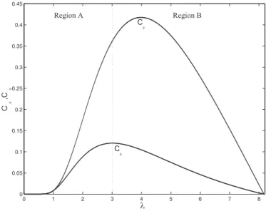
An accurate model for the aerodynamic behavior of a WT is often very difficult to obtain due to the uncertainties in its description. The aerodynamic behavior of the WT is nonlinear, dependent of wind speed and may change over time due to contamination of blade surfaces. In general, the best approach to evaluate the aerodynamic torque Qa uses dimensionless coeffi -cients Cp and Cq, which respectively express the WT ability to convert kinetic energy of moving air into mechanical power or torque [8,19]. Besides dependency of constructive aspects of the WT blades, both coef_ficientsCpandCqare nonlinear functions of the yaw angle

q

and a parameter known as tip-speed ratio

l

, which is defined as:

l

¼ R

u

t

V (8)

where R¼turbine radius,

u

t¼WT speed and V¼wind speed. Admitting that WT is always aligned with wind direction, i.e.

q

¼0_, the aerodynamic torqueQain a blade of WT is given by[8,11,15]:

Qa ¼

1 2

r

AR

Cpð

l

Þ

l

V

2 _¼ 1

2

r

ARCqð

l

ÞV

2 ₍₉₎

where

r

¼air density andA¼rotor area. TypicalCp

l

andCq

l

characteristics of a WT are shown in theFig. 3.

2.3. Driven train

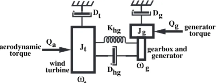
The driven train can be modeled as a set of masses coupled through_flexible connections as shown inFig. 4 [8,20]. Although the gear-box has nonlinear characteristics[21], this component can be supposed ideal. Using the classical rotational dynamics to describe the coupling system of a WT withnblades:

i-th blade:

Ji

u

_iþDi

u

i ¼ Qai Dihð

u

i

u

hÞ Qmih (10)

hub:

J_h

u

__hþD_h

u

_h ¼ X

n

i¼1

½D_ihð

u

_i

u

_hÞ þQ_mihŠ D_hg

u

_h

u

g Qmhg

(11)

electrical generator:

Jg

u

_gþDg

u

g ¼ Dhg

u

h

u

gþQmhg Qg (12)

shaft torques:

_

Q_mih ¼ K_ihð

u

_i

u

_hÞ (13)

_

Qmhg ¼ Khg

u

h

u

g (14)

where

u

i¼i-th blade speed,

u

h¼hub speed,

u

g¼generator speed,

Ji¼i-th blade inertia,Jh¼hub inertia,Jg¼generator inertia (including the gear-box inertia),Di¼i-th blade damping,Dh¼hub damping,

Dg¼generator damping,Dih¼i-th blade-hub connection damping,

Dhg¼shaft damping, Kih¼i-th blade-hub connection stiffness,

Khg¼shaft stiffness,Qai¼i-th aerodynamic torque,Qmih¼i-th blade torque,Qmhg¼shaft torque andQg¼generator torque.

2.4. Electrical generator

The electrical generator constitutes the link between the rota-tional mechanical energy and the available electrical power to

Fig. 3.Aerodynamic characteristics of a WT. R. Rocha / Renewable Energy 36 (2011) 132e141

costumers. Since the dynamics of electrical systems are extremely fast when compared to mechanical coupling, a quasi-static model can be assumed for electrical generator. Considering the use of a current controlled static converter as the interface between the generator and the electrical load, the generator torque Qg is perfectly adjustable in all operating bandwidth and virtually independent from WECS dynamics [8], consisting in the only control input of a stall regulated WT.

3. Nominal linearized model for control design

For robust control design, it is necessary to derive a simplified and linearized mathematical model of the WT. Observing the typical characteristicCq

l

of a WT shown inFig. 3, two distinct operating regions can be identified[8,22,23]:

The stall region (A), characterized by a positive slope of the curveCq

l

, where the operation is unstable and a sudden and significant drop in the aerodynamic torque occurs due to phenomenon known as aerodynamic“stall”;

The normal operation region (B), characterized by a negative slope of the curveCql, which corresponds to normal oper-ation of WT.

The linearization of the aerodynamic torque Qa can be per-formed in the speci_fic point of maximumCp, which is always sit-uated in the normal operating region. In this operating point,

l

¼

l

optand the derivativesvCp/v

u

tandvCp/vVare null. The linear-ized aerodynamic torqueQaaround maximumCpis given by:

_

Qa ¼

a

V_þ

g

u

_t (15)

where

a

is the scaling factor of the torque disturbance due to wind variations_V_, and

g

denotes the acceleration feedback coef_ficient from drive-train. In steady state,V_ is the windfluctuation, which can be assumed as an uncorrelated in the time zero-mean Gaussian stochastic signal[11]. ConsideringVas the nominal wind speed, the coefficients

a

and

g

can be computed from WT data as:

a

¼ v_vQa

Vjlopt

¼ 3

2

r

AR

Cpmax

l

opt

V (16)

g

¼ vQa

v

u

tjlopt

¼ 1

2

r

AR

2Cpmax

l

2_opt V (17)

Although a real mechanical drive train has rigid disks connected by aflexible shaft, where the inertias and compliances are distrib-uted along its length, an approximated lumped 2-mass model pre-sented in Fig. 5 is enough to obtain a good indication of the dynamical loads for control design[8,15]. Admitting an ideal gear-box and reducing all quantities to primary side, the mechanical coupling can be described using classical rotational dynamics[12]:

Jt

u

_tþDt

u

t ¼ Qa Qmhg Dhg

u

t

u

g (18)

Jg

u

_gþDg

u

g ¼ Dhg

u

t

u

gþQmhg Qg (19)

_

Q_mhg ¼ K_hg

u

t

u

g (20)

where

u

t¼WT speed, Jt¼total WT inertia and Dt¼total WT damping.

The structural dynamics and the nonlinearities can be admitted as uncertainties. Thus, the nominal linearized state model of a stall regulated WT for control design is given by:

_

xðtÞ ¼ AxðtÞ þbQgðtÞ þ

j

(21)

yðtÞ ¼ cxðtÞ þ

x

(22)

wherexðtÞ ¼ ½Qa

u

t

u

g QmŠ0and the disturbance input on the system due to wind_fluctuationV_ is given by

j

¼ ½

a

V_0 0 0Š0. Due to practical constraint relatives to assembling, cost and mainte-nance of sensors, the generator rotation

u

g, contaminated by the measurement noise

x

, is considered the only measured outputy. The matricesA,bandcare given by:

A ¼ 2 6 6 6 6 6 4 g Jt

gðDtþDhgÞ Jt

gDhg Jt

g

Jt 1

Jt

DtþDhg Jt

Dhg Jt

1 Jt

0 Dhg

Jg

DhgþDg Jg

1 Jg

0 Khg Khg 0

3 7 7 7 7 7 5

b ¼ h0 0 1 Jg 0

i0

c ¼ ½0 0 1 0Š

4. Some control requirements

For medium- to large-scale systems, the controller design can be dif_ficult from a numerical point of view, since the involved matrix operations tend to be ill-conditioned[4]. Although both speed and power can be selected as the controlled variable in a WECS, the speed control is considered dynamically better than the power control[24]. In this case, the WECS must be operated atfixed

l

optto maximize the energy conversion. This strategy can compromise the control performance due to the direct dependence of the rotation reference with the wind speed, which is always varying and can not be measured exactly at the WT rotor.

Another problem in a WECS is the propagation of vibrations and ripple torque on the system with undesirable consequences on energy quality and lifetime of several system components. Sudden variations in the wind can excite torsional modes, which can cause unacceptable mechanical efforts on the drive train. Although the aerodynamic stall provides the speed limitation for high wind speed, it is necessary to avoid operation in the stall region in order to obtain a better WECS performance[15]. Thus, the control design has to establish a trade-off between the dynamical loads in the system and the increase of the energy conversion. Given the multiple aspects of WECS global ef_ficiency (reliability, availability,

remote operation, quality of captured power, etc.), the WECS optimal control implies the necessity of adopting mixed-criteria optimization indices[25].

The poles of the closed-loop system must be assigned as far away as possible from the frequencies related to the greatest energy density of dynamical loads. Furthermore, it is necessary to obtain suf_ficient gain and phase margins to assure a safe stability margin, since the WECS uncertainties can not be quantified due to the complexity of interactions between WT and windfield. According to Leith e Leithead[12], practical experience suggests that a gain margin of 10 dB and a phase margin of roughly 60_{are sufficient to} assure the control design robustness for any WECS.

5. LQG/LTR methodology

The discrete-time LQG/LTR methodology consists in the formal establishment of a quadratic performance index to synthesize a linear feedback regulatorKc. Considering a discrete-time state model (

F

,

G

,

J

,

P

), the Linear Quadratic Regulator (LQR) provides a control signal that minimizes the following cost function[7,26]:

J ¼ X N

k¼0

½z0ðkÞQzðkÞ þu0ðkÞRuðkފ (23)

where z(k) corresponds to target outputs. The targets and the control input are weighted respectively by matricesQandR, and the resulting discrete-time regulatorKcis given by:

Kc ¼ Rþ

G

0P

G

1

G

0P

F

(24)

wherePis the definite positive solution of the following discrete-time Riccati equation:

P ¼ Qþ

F

0P

F

F

0P

G

Rþ

G

0P

G

1

G

0P

F

(25)

Since the LQR provides a infinite gain margin and at least 60_for phase margin[7], which is enough to assure the WECS stability, the regulator design can be concentrated in to obtain an effective performance for dynamical response. An adequate choice of targets zand weighting matricesQandRallows to establish a quadratic performance index of the LQR similar to the cost function for WECS control described by Leithead et al.[3], which involves the trade-offs between efficiency on energy conversion and the dynamical loads.

The optimization of the energy conversion is an important control requirement for variable speed WECS, and depends on the accuracy of speed control. Thus, the speed error

3

¼

u

ref

u

gcan be used as an indication of efficiency conversion, and its inclusion in the LQR performance index implies a model expansion. In this way, the state model given by eqs.(21) and (22)is discretized for (Ad, Bd, Cd, Dd) and augmented to insert the speed error

3

as a new state variable. The following discrete-time state model is then obtained:

xðkþ1Þ ¼

F

xðkÞ þ

G

QgðkÞ (26)

yðkÞ ¼

J

xðkÞ (27)

where

3

(k) is the discrete summation of the speed error, the new state vector isxðkÞ ¼ ½

3ðkÞ

x0_{ðkÞ Š}0_{andyðkÞcorresponds to new} output. For discrete-time LQG/LTR controller design, the inclusion of this integral action assures the elimination of steady state errors. Hence the discrete-time matrices

F

,

G

and

J

are given by:

F

¼

1 C_dA_d

041 Ad

Jt J g Dt Dg wind turbine gearbox and generator K Dhg hg aerodynamic torque Qa generator torque Qg

ω

ω

t g

Fig. 5.Approximated lumped drive train model.

G

¼ ½ CdBd BdŠ0

J

¼ ½1 014Š

Another important control requirement is to minimization of the detrimental dynamical loads, which are basically determined by mechanical torques and speeds. One of these dynamical loads are the torsional modes, which depend on the difference

D

u

¼

u

t

u

g. To reduce the stress on the shaft, the variations on the shaft torqueQsmust be minimized over all bandwidth. The control design has also to minimize the effects of wind fl uctu-ation and ripple torque over the energy delivered to electrical load, which is represented in the WECS model by the generator torque Qg. Thus, the targets can be chosen as zðkÞ ¼MxðkÞ, where the matrix Mis:

M ¼ 2 6 6 6 6 4

1 0 0 0 0

0 0 1 1 0

0 0 1 0 0

0 0 0 1 0

0 0 Dhg Dhg 1

3 7 7 7 7 5

Since the weighting matrices are selected asQ¼diag(w1,w2,w3,

w4,w5) andR¼w6, the performance index of the LQR regulator is

converted into:

J ¼X N

0 h

w1ð

3

Þ2þw2ð

D

u

Þ2þw3ð

u

tÞ2þw4

u

g2

þw5ðQsÞ2þw6Qg2

i

ð28Þ

The relative importance of each target on the index to be minimized by the LQR action is determined by its respective weight wi, which establishes the intensity of the control action on a spec-i_fied target. The use of weights dependent on frequency (weighting functions) increases theflexibility on targets manipulation, allow-ing to penalize selectively a determined bandwidth. However, weighting functions increases the controller complexity due to addition of extra dynamics to the original model. The selection of the weightswidepends strongly on the system configuration and the inevitable design trade-offs.

The complement of the LQG/LTR controller design consists in the determination of the discrete-time Kalmanfilter for optimal esti-mation of the state variables, which will be used as the exact measurements by LQR. This_filter estimates the state vectorbxðk=kÞ from actual measurement vectory(k), taking the following form[27]:

b

xðkþ1=kÞ ¼

Fb

xðk=k 1Þþ

G

uðkÞ

F

Kf

Jb

xðk=k 1Þ yðkÞ

(29)

b

xðk=kÞ ¼ bxðk=k 1Þ Kf

Jb

xðk=k 1Þ yðkÞ (30)

Assuming the state and measurement noise covariance matricesW andV,Kfis given by:

Kf ¼ P

J

0

J

P

J

0þV 1 (31)

where P is the positive semidefinite solution of the Riccati equation:

P ¼

F

P

F

0

F

P

J

0

J

P

J

0þV 1

J

P

F

0þW (32)

The complete WECS controller is synthesized by connection of the Kalmanfilter to LQR, as shown inFig. 6. However, the inclusion of the Kalman_filter can imply in the degradation of robustness and performance properties obtained in the LQR design. It is possible to recover these properties through the LTR procedure (Loop Transfer Recovery), which consists in an adequate choice of the covariance matricesVandWin the Kalman_filter design[6,7,27]. This proce-dure also allows the asymptotic closed-loop poles placement, avoiding undesirable frequencies[26].

6. Sensorless control

For maximum energy conversion, the speed reference

u

refmust be directly proportional to wind speed to assure the WT operation at

l

opt. This strategy can reduce the control robustness due to problems related to wind speed measurement. However, the optimal speed reference

u

reffor the control system can be indirectly obtained, avoiding the necessity to measure the wind speed. From eq.(9), the following relationship is obtained considering the WECS operating at

l

opt:

u

_ref ¼ Kqa

ffiffiffiffiffiffi

Qa p

(33)

whereKqais a constant value given by:

Kqa ¼

l

opt_R

ffiffiffiffiffiffiffiffiffiffiffiffiffiffiffiffiffiffiffiffiffi

2

l

opt

r

ARCpmax

s

(34)

Since the aerodynamic torque Qa measurement is not directly available, it is estimated from the preceding data using a Kalman predictor, as shown the Fig. 7. Considering the nominal WECS model described in section 2, the dynamics of the Kalman predictor is given by eq. (29), where the gain Kf is computed using the eqs.(31) and (32) [27]. The covariance matricesWand V must be selected for a slowest response if compared to feedback controller, aiming a good filtering of the speed refer-ence and the decoupling between predictor and controller dynamics.

There are several proposed strategies for the elimination of a sensor to measure the shaft speed of an electrical motor that can used in the case of the generator. The most of these

strategies is based in the estimative of back emf (in the case of the generator, emf), a phenomenon that depends of the rotor speed which can be estimated from the machine voltage and current measurements [28e31]: from a dynamical model, an adaptive observer is designed to estimate the states and the rotor speed. The drawback of this strategy is its inherent dependence with the machine parameters, which becomes the speed estimation sensible to parameter uncertainties [32]. The second strategy is the injection of a high frequency voltage wave in the machine terminals to induce a current signal, which depends of the rotor position [33]. However, this strategy requires constructive modifications in the machine aiming to avoid torque pulsation [32]. The third strategy consists in the monitoring of the harmonic components produced by rotor slots, which filtering provides signal equivalent to an incremental encoder which resolution is p(Nrþ1) pulses per revolution, wherep¼number of pole pairs of the machine andNr¼number of slots per pole pairs [34].

7. Simulation results

The performance of the proposed sensorless control structure is verified from computational simulations considering a Hori-zontal Axis WT shown in theFig. 8with two blades of 45.72 m

each, which normalized data in relation to its rated values (2.5 MW and 17 RPM) are presented in Table 1. The WECS is simulated using the nonlinear model presented in section 2. The control structure is designed using the nominal linearized model described in section 3, considering a sample interval ofTs¼5 ms and a nominal wind speed ofV ¼6:7m=s. The weights for LQR are chosen as w1¼500, w2¼500, w3¼100, w4¼100, w5¼100

andw6¼1. The covariance matrices for the Kalmanfilter design

are selected asV¼

3

j

0

_j

_andW¼10 3_{. Using the LTR procedure,}

the parameter

3

is adjusted to 105 _{to obtain a good properties}

recovery. The Kalman predictor is designed selecting the covariance matrices as Vpred¼Ts2

jj

0 and Wpred¼

a

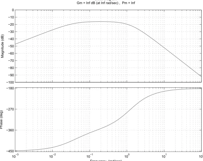
2. The frequency response of the open-loop control system can be veri_fied by Bode diagrams shown in Fig. 9, where the in_finite gain and phase margins indicate a stable close-loop control system.

The_first simulated event is the wind gust shown in Fig. 10. Its is observed inFig. 11that the LQG/LTR controller provides an accurate adjustment for generator speed

u

g. Thus, the WECS operates practically closed at constant

l

as shown in Fig. 12. Since system losses are not considered, the speed reference obtained by the Kalman predictor is slightly below the ideal reference. None torsional mode is excited by this wind gust. The control system imposes an adequate attenuation for wind fl u-tuaction and ripple torque, avoiding the propagation of dynamical loads to other parts of the WECS, as can be observed inFigs. 11 and 13.

Since a WT can be submitted to sudden wind variations, the second simulated event to verify the closed-loop dynamics is a wind step. Considering the operation at a mean wind speed of 6.7 m/s, it is suddenly varied to 8.9 m/s after 20 s as shown the Fig. 14. In face of the increase on wind speed, the controller increases the generator speed (Fig. 15) to maintain

l

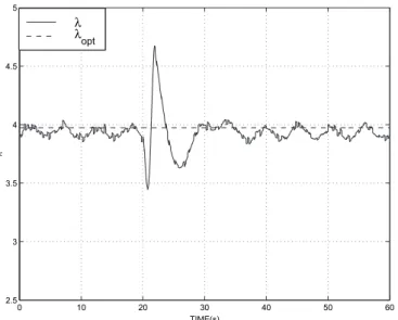
constant (Fig. 16), assuring the WECS operation almost in maximum effi -ciency on energy conversion. None torsional mode is excited by this wind step. It is observed inFigs. 15 and 17that the control system continues imposing an adequate attenuation for windflutuaction and ripple torque for a wind speed of 8.9 m/s. In this context, the fatigue on drive-train components is reduced, improving the quality of generated energy.

Fig. 7.Sensorless controller for WT: Optimal speed reference determination.

Table 1

WT normalized data.

Jt¼37.413 Dt¼2.02410 2

Khg¼28.4 Dhg¼1.831

Jg¼2.091 Dg¼3.0110 2

Fig. 8.Horizontal Axis WT used in computational simulations.

−100 −90 −80 −70 −60 −50 −40 −30 −20 −10 0

Magnitude (dB)

10−3 10−2 10−1 100 101 102

−450 −360 −270 −180

Phase (deg)

Bode Diagram

Gm = Inf dB (at Inf rad/sec) , Pm = Inf

Frequency (rad/sec)

Fig. 9.Bode diagrams for open-loop WECS control system.

0 10 20 30 40 50 60

6.5 7 7.5 8 8.5

TIME(s)

WIND SPEED(m/s)

Fig. 10.Wind gust.

0 10 20 30 40 50 60

0 0.05 0.1 0.15 0.2 0.25

TIME(s)

SPEED

ω t ω

g ω

ref

0 10 20 30 40 50 60 2.5

3 3.5 4 4.5 5

TIME(s)

λ

λ λ

opt

Fig. 12.Tip-speed ratio for the wind gust.

0 10 20 30 40 50 60

0 0.5 1 1.5 2 2.5 3 3.5 4 4.5 5

TIME(s)

TORQUE

Q_a Q_g Q_s

Fig. 13.Torques for the wind gust.

0 10 20 30 40 50 60

6.5 7 7.5 8 8.5 9

TIME(s)

WIND SPEED(m/s)

Fig. 14.Wind step.

0 10 20 30 40 50 60

0 0.05 0.1 0.15 0.2 0.25

TIME(s)

SPEED

ω t ω

g ω

ref

Fig. 15.Normalized speeds for a step on wind speed.

0 10 20 30 40 50 60

2.5 3 3.5 4 4.5 5

TIME(s)

λ

λ λ

opt

Fig. 16.Tip-speed ratio for a step on wind speed.

0 10 20 30 40 50 60

0 0.5 1 1.5 2 2.5 3 3.5 4 4.5 5

TIME(s)

TORQUE

Q a Q

g Q_s

Fig. 17.Torques for a step on wind speed. R. Rocha / Renewable Energy 36 (2011) 132e141

8. Conclusions

This paper presents a sensorless control for a variable speed WT operating at partial load, that feeds an electrical load through static power converters. The speed reference is obtained from a Kalman predictor, which estimates the aerodynamic torque and avoids the direct wind speed measurement. This procedure is very attractive, since the complexity and the uncertainty of wind measurement can compromise the robustness of the control system. The LQG/LTR methodology was applied to design an optimal discrete-time feedback controller for a WECS. Since this methodology automati-cally assures the stability margin for the close-loop system, the control system is designed to obtain an effective performance for dynamical response through an adequate choice of targets and weighting matrices, establishing a formal cost function to be minimized by control action. The objective is to increase the effi -ciency on energy conversion, reducing the detrimental dynamic loads caused by windfluctuation and ripple torque. Considering a consistent nonlinear dynamical model for WT system as the real plant, a wind gust and a step variation on wind speed are simulated to verify the closed-loop system performance. The simulation results have shown that the proposed sensorless control structure provides a WECS operation near the maximum ef_ficiency point, reducing the influence of vibrations and ripple torque and, conse-quently, the stress over the mechanical drive system.

Acknowledgments

The authors gratefully acknowledge the_financial support of the National Counsel of Technological and Scienti_fic Development (CNPq), State of Minas Gerais Research Foundation (FAPEMIG), Gorceix Foundation and Federal University of Ouro Preto.

References

[1] Lefevbre S, Dubé B. Control system analysis and design for an aerogenerator with eigenvalue methods. IEEE Trans Power Syst 1988;3(4):1600e8. [2] Dessaint L, Nakra H, Mukhedkar D. Propagation and elimination of torque

ripple in a wind energy conversion system. IEEE Trans Energy Conversion 1986;1(2):104e12.

[3] Leithead WE, de la Salle S, Reardon D. Role and objectives of control for wind turbines. IEE Proc Pt C 1991;138(2):135e48.

[4] Østergaard K, Stoustrup J, Brath P. Linear parameter varying control of wind turbines covering both partial load and full load conditions. Int J Robust Nonlinear Control 2009;19:92e116.

[5] Geng H, Yang G. Robust pitch controller for output power levelling of variable-speed variable-pitch wind turbine generator systems. IET Renewable Power Generation 2009;3(2):168e79.

[6] Grimble MJ. Robust industrial control - optimal design approach for poly-nomial systems, systems and control engineering. New York: Prentice Hall International; 1994.

[7] Maciejowski JM. Multivariable feedback design. Wokingham, England: Addi-son-Wesley Publishing Company Inc.; 1989.

[8] Novak P, Ekelund T, Jovik I, Schmidtbauer B. Modeling and control of variable-speed wind-turbine drive-system dynamics. IEEE Control Syst 1995;15 (4):28e38.

[9] Leithead WE. Variable speed operation - does it have any advantages? Wind Eng 1989;13(6):302e14.

[10] Rocha R, Resende P, Silvino J.L, Bortolus M.V. Control for a wind turbine without wind measurement. In: Proceedings XVI COBEM, ABCM, Uberlândia, Brazil; 2001.

[11] Wasynczuk O, Man DT, Sullivan JP. Dynamic behaviour of a class of wind turbine generators during random windfluctuations. IEEE Trans. Power Apparatus Syst 1981;100(6):2837e45.

[12] Leith DJ, Leithead WE. Implementation of wind turbine controllers. Int J Control 1997;66(3):349e80.

[13] Rohatgi J, Pereira A. Modeling wind turbulence for the design of large wind turbines - a preliminary analysis. In: IV CEM-NNE; 1996. p. 735e9. [14] Anderson PM, Bose A. Stability simulation of wind turbine systems. IEEE Trans

Power Apparatus Syst 1983;102(12):3791e5.

[15] Freris LL, editor. Wind energy conversion systems. United King: Prentice Hall Inc.; 1990.

[16] Golding EW. The generation of electricity by wind power. London, UK: E. & F.N. Spon LTD; 1977.

[17] Raina G, Malik OP. Variable speed wind energy conversion using synchronous machine. IEEE Trans Aerospace Electronic Syst 1985;21(1):100e4. [18] Hwang HH, Gilbert LJ. Synchronization of wind turbine generators against an

infinite bus under gusting wind conditions. IEEE Trans Power Apparatus Syst 1978;97(2):536e44.

[19] Medeiros A, Simões FJ, Lima AMN, Jacobina CB. Modelagem aerodinâmica de turbinas eólicas de passo variável. Florianópolis, Brazil: VI ENCIT/VI LATCYM, ABCM; 1996. pp. 25e30.

[20] Hori Y, Sawada H, Chun Y. Slow resonance ratio control for vibration suppression and disturbance rejection in torsional system. IEEE Trans Ind Electronics 1999;46(1):162e8.

[21] Lefebvre S, Dessaint L, Dubé B, Nakra H, Pérocheau A. Simulator study of a vertical axis wind turbine generator connected to a small hydro network. IEEE Trans Power Apparatus Syst 1985;104(5):1095e101.

[22] Rocha R, Resende P, Silvino J.L, Bortolus M.V. Control of stall regulated wind turbine through HNloop shaping method. In: 2001 IEEE conference on control applications CCA2001, vol. 1. Mexico City; 2001. p. 925e9. [23] Rocha R, Martins Filho L.S. A multivariable HN control for wind energy

conversion system. In: 2003 IEEE conference on control applications CCA2003, vol. 1. Istambul; 2003. p. 206e11.

[24] Hinrinchsen E, Nolan P. Dynamics and stability of wind turbine generators. IEEE Trans Power Apparatus Syst 1982;101(8):2640e8.

[25] Bratcu A, Munteanu I, Ceangã E. Optimal control of wind energy conversion systems: from energy optimization to multi-purpose criteriaea short survey. In: 16th Mediterranean conference on control and automation. Ajaccio, France; 2008. p. 759e66.

[26] Anderson BDO, Moore JB. Optimal controlelinear quadratic methods. New Jersey, USA: Prentice Hall Inc.; 1990.

[27] Maciejowski JM. Asymptotic recovery for discrete-time systems. IEEE Trans Automatic Control 1985;30(6):602e5.

[28] Bose B. Power electronics and variable frequency drives: technology and applications. IEEE Press; 1997.

[29] Lefley P.W, Peasgood W, Ong R, Wong J.K.J. Sensorless close loop control of a slip ring induction machine using adaptive signal processing. In: 14th annual applied power electronics conference and exposition, APEC99; 1999. [30] Cárdenas R, Peña R, Asher G, Cilia J. Sensorless control of induction machines

for wind energy applications. In: 33rd annual power electronics specialists conference, PESC2002; 2002.

[31] Cárdenas R, Peña R, Asher G, Clare J. Power smoothing in wind generation systems using a sensorless vector controlled induction machine driving aflywheel. IEEE Trans on Energy Conversion;19(1).

[32] Hilairet M, Auger F. Frequency estimation for sensorless control of induction motors. In: Proceedings of 2001 IEEE conference on acoustic, speech and signal processing; 2001.

[33] Holtz J. Sensorless position control of induction motors e an emerging technology. IEEE Trans on Industrial Electronics;45(6).