doi: 10.1590/0101-7438.2015.035.02.0401
SELECTING PROFILES OF IN DEBT CLIENTS OF A BRAZILIAN TELEPHONE COMPANY: NEW LASSO AND ADAPTIVE LASSO ALGORITHMS IN THE COX MODEL
Marcelo A. Costa
1*, Enrico A. Colosimo
2and Carolina G. Miranda
2Received January 24, 2013 / Accepted November 16, 2014
ABSTRACT.Variable selection plays an important rule in identifying possible factors that could predict the behavior of clients with respect to the bill payments. The Cox model is the standard approach for mod-eling the time until starting the lack of payments. Parsimony and capacity of predicting are some desirable characteristics of statistical models. This paper aims at proposing a new forward stagewise Lasso (least ab-solute shrinkage and selection operator) algorithm and applying it for variable selection in the Cox model. The algorithm can be easily extended to run the Adaptive Lasso (ALasso) approach.
Keywords: proportional hazards model, partial likelihood, lasso regression.
1 INTRODUCTION
The cell phone market has grown fast in recent years. Modern cell phones, advantageous plans and services provided by the telephone companies have attracted new clients. Also due to the variety of companies with competitive services, the clients may change their telephone provider. One of the greatest challenges faced by telephone companies, which were generated by such a huge expansion in the market, is to identify the characteristics of their new and current clients. It is in the company’s interest to attract faithful clients, or in a different perspective, to identify the profile of in debt clients. This is imperative in order to define new politics which leads the company to increase and to offer its clients more appropriate and specific services such as pre-paid services.
In debt clients are either clients who start the service and do not pay their bill or who stop pay-ments after a certain time. In both cases, the time until the lack of paypay-ments is the response
*Corresponding author.
1Department of Production Engineering, Universidade Federal de Minas Gerais, Belo Horizonte, MG, Brazil. E-mail: [email protected]
variable. The goal is then to identify possible factors related to the client’s socioeconomic con-ditions, the service provided by the company, among others that could predict the behavior of the clients with respect to bill payments. In this context, survival analysis and variable selection techniques are the common tools to handle the problem.
Survival analysis involves the study of response times from a well defined point in time to a pre-specified outcome event and, in general, the interest focuses on the effect of covariates on survival. Statistical analysis is often complicated by the presence of incomplete or censored ob-servations in data sets. That is, frequently, the failure event is not observed for some subjects by the end of follow-up or it is not observed exactly but, in such cases, it is known that it occurred in a certain period of time. Literature in survival analysis has been increasing enormously after the seminal work of Cox [1, 2] on the proportional hazards model. Classical texts include Cox & Oakes [3], Kalbfleish & Prentice [4] and Lawless [5].
The most popular expression of Cox regression model, for covariates not dependent on time, uses the exponential form for the relative hazard, so that the hazard function is given by:
λ(t)=λ0(t)exp(βTx), (1)
whereλ0(t), the baseline hazard function, is an unknown non-negative function of time,βT =
(β1, . . . , βp)is a p×1 vector of unknown parameters andx = (x1, ...,xp)T is a row vector
of covariates. Inference forβis usually based on the partial log-likelihood function, taken into consideration a sample ofnindividuals, in which it is observedk≤nfailures at timest1≤t2≤ · · · ≤tk. In the absence of ties, for the model (1), this function is written as:
l(β)=
n
i=1
δi
⎡
⎣βTxi−log
⎛
⎝
jεR(ti)
exp(βTxj)
⎞ ⎠ ⎤
⎦ , (2)
whereδi is the failure indicator andR(ti) is the set of labels related to the individuals at risk at
timeti.
An alternative procedure that has shown a nice variable selection performance is the Lasso (Least Absolute Shrinkage and Selection Operator) method proposed by Tibshirani [12]. This technique has attracted attention in the literature mainly due to its capability as providing automatic variable selection and optimized prediction performance. Some properties of it are presented by Knight & Fu [13]. An estimate of the shrinkage parameter was proposed by Foster et al. [14] by using a random linear model approach. In special for the Cox model, Tibshirani [15] applied the Lasso method for variable selection. Recently, adaptive Lasso methods have been proposed by Zhang & Lu [16] and Zou [17] for the proportional hazards model. These methods consider adaptive penalizations for the regression coefficients.
Originally, the Lasso method requires a Newton-Raphson step in its iteractive process [15]. This is a really difficult step especially in the presence of many covariates. Recently, Friedman et al. [18] proposed a fast algorithm namedglmnetto estimate the Lasso solutions based on the Coordinate Descent algorithm [19]. Simon et al. [20] extended the Coordinate Descent algorithm to the Cox model.
This paper aims at proposing a new Lasso algorithm for variable selection in Cox model as a non-linear extension of theForward stagewise linear regressionalgorithm Tibshirani et al. [21]. The algorithm presents good performance for this model and it can be easily extended for other sorts of models. Furthermore, the proposed algorithm can be extended to generate ALasso (Adaptive LASSO) estimates. The ultimate goal is to identify characteristics of the in debt clients of a Brazilian telephone company.
The structure of the present paper is as follows. The Lasso method is described in Section 2. Section 3 presents the original algorithm proposed by Tibshirani [15]. The Forward Stagewise Lasso algorithm is presented in Section 4 and also an extended version which generates ALasso solutions. Monte Carlo simulations are used in Section 5 in order to compare Lasso, ALasso and other variable selection techniques. In Section 6, variable selection techniques are applied to the data set reported in Fleming and Harrington [22]. The Brazilian telephone company data set is analyzed in Section 7. Discussion and Conclusion in Section 8 ends the paper.
2 THE LASSO METHOD
The Lasso method was proposed by Tibshirani [12]. It is originally aimed at minimizing the constrained residual sum of squares (error) where the constraint is represented by the sum of the absolute coefficients function as shown in the following:
ˆ
βlasso = arg min
β N
i=1
yi−pj=1xi jβj
2
,
subject to : pj=1|βj| ≤s.
(3)
where yi is the response for thei-th individual in the sample, which is usually assumed to be
normally distributed, ands is the Lasso parameter whose maximum value is associated to the standard least squares estimatess0=pj=1| ˆβlsj |. The method is very similar to the norm
algorithm is also able to provide coefficients that are exactly zero, therefore providing variable selection. In addition, it minimizes multi-collinearity and consequently leads to the improvement of the model prediction performance.
The Lasso method was previously used for variable selection in the Cox model [15] to maximize the partial likelihood subjected to the same constraint function presented in (3), that is,
ˆ
βlasso = arg max
β l(β),
subject to : pj=1|βj| ≤s.
(4)
It can be noticed from (3) and (4) that the solution depends on the constraint values or Lasso parameter, which must be chosen based on some quality measures. Originally, quality measures such as cross-validation, generalized cross-validation and analytical unbiased estimate of risk were used for linear models [12] and an approximated generalized cross validation statistic for the Cox model [15]. In all these cases an approximation for the number of parameters involved in the fittedβˆlassois calculated using matrix algebra, which can be a hard task.
In addition, Leng et al. [24] reported that prediction accuracy criterion is not suitable for vari-able selection using the Lasso method. Results were provided for linear regression models only. Alternatively, we propose and evaluate the use of BIC (Bayesian Information Criteria) as the optimization function for selecting the Lasso parameter.
2.1 The adaptive LASSO (ALASSO)
Zhang & Lu [16] proposed a weighted L1penalty on the regression coefficients such that the estimates can be found by solving the following maximization problem,
ˆ
βalasso = arg max
β l(β),
subject to : pj=1|βj|/| ˆβ∗j| ≤s.
(5)
whereβˆ∗j is the maximizer of the log partial likelihood,l(β). According to Zhang & Lu [16], the ALasso approach has the desired theoretical properties and computational convenience. In this work, we found that our algorithm can be extended to generate ALasso solutions. It is also worth noting that by including a weighted penalty, the ALasso estimates exclude parameters with low absolute values, and it therefore generates more compact models when compared to the original Lasso estimates.
3 THE ORIGINAL LASSO ALGORITHM
Tibshirani [15] proposes an algorithm to obtain Lasso estimates as an adaptation of the Newton-Raphson iterative least squares algorithm. Let η= Xβ be the linear predictor, where X is the regression matrix,β is the coefficients vector. Letu =∂l/∂ηandA = −∂2l/∂ηηT. Consider W asW =diag{aii}the diagonal matrix whose elements are the diagonal components ofAand
Step 1 Fixsand start withβˆ=0.
Step 2 Computeη,u,Aandzfromβˆ.
Step 3 Minimize(z−Xβ)TW(z−Xβ)subject topj=1|βj| ≤s.
Step 4 Repeat Steps 2 and 3 untilβˆdoes not change.
To perform Step 3, consider such minimization problem as a weighted least squares problem subjected to a general linear inequality constraint, say,
Minimize(z−Xβ)TW(z−Xβ), subject toCβ≤ D,
for some matricesCandD. This approximation leads to the following solution:
β = ˆβ+(XTW X)−1CT
C((XTW X)−1)CT −1
(D−Cβ),ˆ (6)
whereβˆ=(XTW X)−1XTW z.
Instead of applying 2p possible constraints representing all possible combinations of signals for the parametersβ, Lawson & Hansen [25] suggest to grow matricesC andD, sequentially, starting withD = s andCT = sign(βˆ0), wheresign()is the signal function,βˆ0 is the non-constraint solution and from Equation 6 find a new estimateβ. Ifj=1|βj|>sinclude a new
linei in matricesC andD withCiT =sign(β ), D =s1,1 =(1, . . . ,1)T, and obtain a new solutionβk+1. The procedure stops at stepk,k=1,2, . . . ,m, whenj=1|βj| −s< ξ, whereξ
is the numerical tolerance, andmis the maximum number of steps. Both,ξandm, are specified by the user.
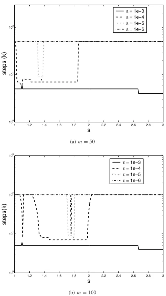
Results show that for a particular range ofsthe algorithm reaches the tolerance before reaching the maximum number of steps. As the tolerance decreases, the algorithm stops when it reaches the maximum number of steps. Therefore, the algorithm is not capable of generating solutions if the tolerance is below a certain threshold, in this example this threshold is approximately 10−4. Figure 1(b) shows that even when selecting a higher number of steps (m=100) the convergence problem remains.
1 1.2 1.4 1.6 1.8 2 2.2 2.4 2.6 2.8 3 100
101 102
s
steps (k)
ε = 1e−3 ε = 1e−4 ε = 1e−5 ε = 1e−6
(a)m=50
1 1.2 1.4 1.6 1.8 2 2.2 2.4 2.6 2.8 3 100
101 102 103
steps(k)
s
ε = 1e−3 ε = 1e−4 ε = 1e−5 ε = 1e−6
(b)m=100
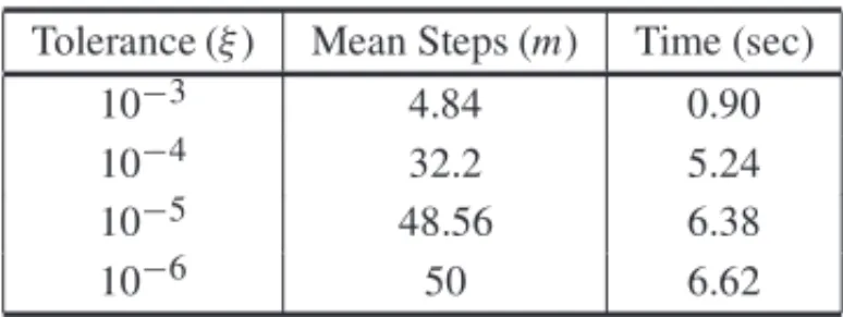
Table 1 shows the average for both, the number of steps for different values of toleranceξ and the computational time for 200 solutions within the previous range ofsas shown in Figure 1(b). According to Table 1 a single solution with tolerance equal to 10−3converges, on average, in 4.84 steps or 0.9 seconds. As expected, for small values ofξ the mean number of steps tends to be close to the maximum number of stepsm. This represents a lower bound for the tolerance not crossed by the algorithm.
Table 1– Mean computational time in seconds for original Lasso algorithm for different values of tol-erance and maximum number of steps equals to 50.
Tolerance (ξ) Mean Steps (m) Time (sec) 10−3 4.84 0.90 10−4 32.2 5.24 10−5 48.56 6.38
10−6 50 6.62
Following Zhang & Lu [16], the ALasso optimization problem is strictly convex and therefore standard optimization packages available, for example, in Matlab and R can be used to generate the estimates. The authors also propose minimizing the penalized log partial likelihood using a variation of the Fu’s shooting algorithm [26].
An alternative approach to solve both Lasso and ALasso optimization problems is to use La-grange Multiplier and rewrite the constrained optimization problem as λ·l(β) +(1 −λ)· p
j=1|βj|, for the Lasso estimate, and λ·l(β)+(1 −λ)· p
j=1|βj|/| ˆβ∗j| for the ALasso
estimate. In this case, 0≤ λ ≤1, and therefore estimates might be provided by standard opti-mization packages for different values ofλ. Furthermore, in this case, the Lasso parameter, s, and the Lagrange Multiplier,λ, are related.
4 THE FORWARD STAGEWISE LASSO ALGORITHM
In order to avoid the problems mentioned in the previous section, we proposed a new algorithm that outperforms previous ones since it does not require computing first and second order deriva-tives, and relies on simple programming code based on a test-and-update approach. However, our approach increases the computational burden as compared to previous algorithms, which can be substantially minimized using a more efficient programming language such as C/C++. The algo-rithm is based on theforward stagewise linear regression[21]. The coefficients are initiated with zero and a small increment,ǫ, is added to each one of them, separately. The log partial likelihood is then measured and the candidate that maximizes the log-function is updated. The process is continuously repeated until it reaches a maximum number of iterations, say M. The increment
Algorithm
Initializeβˆj =0, j=1, ...,p.
Setǫ >0to some small constant andM large Form=1toM
lmax =l(β)ˆ Forj=1to p
Forx=1to2
ǫ= −ǫ βaux = ˆβ βauxj =βauxj +ǫ Ifl(βaux) >lmaxthen
k∗= j α∗=βauxj lmax=l(βaux) end If
end For end For
ˆ
βk∗=α∗ end For end Algorithm
Figure 2– Forward Stagewise Lasso algorithm.
Despite increasing computational cost with such a test-and-update approach, it is remarkable the simplicity of the proposed algorithm and its capability of generating approximations of the Lasso solutions without the need of computing first or second order derivatives. Originally, the Lasso method was applied to the Cox model by means of an iterative Newton-Raphson update [15]. In that case, convergence is quite fast to a single solution, but multitudes of solutions have to be generated in order to select the final one with the proper constraint value for the sum of the absolute coefficients. Consequently, if a high resolution for the constraint is chosen, the compu-tational effort might be greater than that for the proposed algorithm. Moreover, in our simulation study and for the real data fitting, the proposed algorithm did converge to the maximum log-likelihood estimate.
In a very similar way, our proposed Forward Stagewise Lasso algorithm has two parameters the step lengthǫand the maximum number of stepsM. However, these parameters are related to the maximum amount of solutionsMgenerated by the algorithm and the difference between the sum of the absolute coefficients in two consecutive steps i.e.
| ˆβj(k)| −| ˆβj(k−1)|
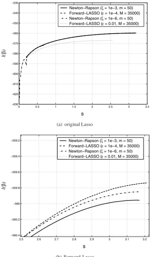
the global maximum. The Forward Stagewise Lasso parameters,ǫandm, when compared to the original algorithm, do not control convergence. However, it is crucial to choose a suitable value forǫotherwise the set of solutions will be biased. Figure 3(a) compares the partial log-likelihood curve for original and the proposed algorithm. Ifǫ = 0.01 the proposed approach generates biased solutions and converges to a local maximum before reaching the maximum number of stepsM =35,000. If changed toǫ=10−4thel(β)curve achieves its maximum with 33,651 steps. Indeed, Figure 3(b) shows that our proposal provides a fine resolution with slightly higher values forl(β) when solutions are closer to the maximum partial likelihood estimate βˆ∗j. In addition, our approach generates on average one single solution in 0.1675 seconds. The 33,651 solutions took approximately 93.94 minutes using a code implemented in Matlab software. It is worth noting that computing speed can be substantially improved using C\C++ language. Although the smaller theǫthe higher the computational cost required to generateM solutions, empirical results have shown that after a certain small valueǫ∗, the set of solutions becomes stable, not differing substantially if an even smallerǫvalue is applied. An empirical approach to select the parameterǫis to execute the algorithm several times, each one with a differentǫvalue.
Comparing both algorithms, the original approach is very sensitive to the number of variables in the model. For a large number of variables such algorithm leads to numerical problems due to difficulties in the calculation of the inverse of matrices. Figure 4(a) shows the estimates for the liverdata set. For small values ofs(s <0.3), the algorithm is not able to generate solutions. Problems with the numerical convergence appear as spikes and non-smooth sequential estimates. However, this algorithm has the advantage of generating fast solutions for arbitrary values ofs. The proposed approach does not present problems with the numerical convergence since no inverse matrices are needed. The estimates are very smooth as noticed in Figure 4(b). However, although it generates one solution much faster than the original approach, we need to estimate a large set of solutions with some relatively fine resolution starting fromβˆj =0 which increases
computational cost considerably.
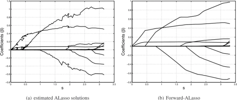
Furthermore, our approach can be extended to generate ALasso solutions. Briefly, the ALasso approach penalizes parameters with low absolute values and it prioritizes the parameters with large absolute values. In our algorithm this feature is implemented by replacing the parameters update step, defined asβauxj =βauxj +ǫ, withβauxj =βauxj +ǫ· | ˆβ∗j|. Figure 5 shows ALasso solutions generated with an optimization package available in R software, as suggested by Zhang & Lu [16], and also the solutions provided by our algorithm. Results show that our approach minimizes instabilities due to numerical approximations.
5 COMPARING LASSO, GLMNET, ALASSO AND OTHER METHODS
FOR VARIABLE SELECTION
0 0.5 1 1.5 2 2.5 3 3.5 −630
−620 −610 −600 −590 −580 −570 −560 −550 −540 −530
s
l(
β
)
Newton−Rapson (ξ = 1e−3, m = 50)
Forward−LASSO (ε = 1e−4, M = 35000)
Newton−Rapson (ξ = 1e−6, m = 50)
Forward−LASSO (ε = 0.01, M = 35000)
(a) original Lasso
2.5 2.6 2.7 2.8 2.9 3 3.1 3.2
−560.4 −560.2 −560 −559.8 −559.6 −559.4 −559.2
s
l(
β
)
Newton−Rapson (ξ = 1e−3, m = 50)
Forward−LASSO (ε = 1e−4, M = 35000)
Newton−Rapson (ξ = 1e−6, m = 50)
Forward−LASSO (ε = 0.01, M = 35000)
(b) Forward-Lasso
Figure 3– Partial log-likelihood as a function ofs for original (Newton-Raphson) and Forward-Lasso algorithms.
0 0.5 1 1.5 2 2.5 3 3.5 −0.8 −0.6 −0.4 −0.2 0 0.2 0.4 0.6 0.8 1 s Coefficients ( β )
(a) original Lasso
0 0.5 1 1.5 2 2.5 3 3.5 −0.8 −0.6 −0.4 −0.2 0 0.2 0.4 0.6 0.8 1 s Coefficients ( β ) (b) Forward-Lasso
Figure 4– Estimates for original Lasso and Forward Lasso algorithms. Numerical approximations to the inverse of matrices leads to convergence problems in the original approach.
0 0.5 1 1.5 2 2.5 3 3.5 −0.8 −0.6 −0.4 −0.2 0 0.2 0.4 0.6 0.8 1 1.2 s Coefficients ( β )
(a) estimated ALasso solutions
0 0.5 1 1.5 2 2.5 3 3.5 −0.8 −0.6 −0.4 −0.2 0 0.2 0.4 0.6 0.8 1 s Coefficients ( β ) (b) Forward-ALasso
Figure 5– Estimates for ALasso and Forward ALasso algorithms. Alasso coefficients were generated using a numerical optimization package available in the R software.
The AIC and BIC measures were applied as variable selection techniques as the following. Given pcandidate variables, all 2p−1 possible combinations were tested. The combinations with the highest AIC and BIC values were compared to the true model.
For theglmnetpackage, we apply theleave-one-outcross-validation to select the Lasso parame-ter.
forρ are assumed: ρ =0.5 (decreasing failure rate), ρ = 1 (constant failure rate) andρ =2 (increasing failure rate). Vectorβ is set equal to(1,0,0,1)or(1,0,0,1,1)for scenarios which consider 4 or 5 covariates, respectively. Covariates are generated from the following distribu-tions: the standard normal (N), the Bernoulli (B) with parameter θ = 0.5, and the exponential (E) with mean equal to 1. The scenarios are described in Table 2.
Table 2– Scenarios for the Monte Carlo study.
Scenario Sample size Percentage of censoring Response variables
1 50 0.0 (N, N, B, B)
2 100 0.0 (N, N, B, B)
3 100 30.0 (N, N, B, B)
4 50 0.0 (N, N, B, B, E)
For each scenario, 5,000 replications generated using the Weibull model are considered and it is calculated the percentage of times that the model is correctly selected by each method and criteria. For the Lasso and ALasso methods, it is also assumedǫ = 0.001 and M = 40,000. MATLAB and R packages were used in order to get the results.
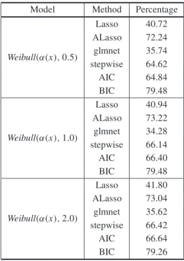
Tables 3 and 4 show the results for Scenarios 1 and 2. From these tables, there may be observed the effect of sample sizes as well as the failure rates in the variable selection, for all methods.
Table 3– Percentage of correct model selection, Scenario 1.
Model Method Percentage
Weibull(α(x),0.5)
Lasso 40.72 ALasso 72.24 glmnet 35.74 stepwise 64.62 AIC 64.84 BIC 79.48
Weibull(α(x),1.0)
Lasso 40.94 ALasso 73.22 glmnet 34.28 stepwise 66.14 AIC 66.40 BIC 79.48
Weibull(α(x),2.0)
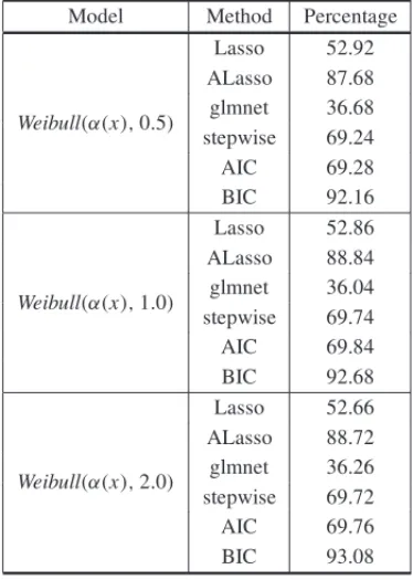
Table 4– Percentage of correct model selection, Scenario 2.
Model Method Percentage
Weibull(α(x),0.5)
Lasso 52.92 ALasso 87.68 glmnet 36.68 stepwise 69.24 AIC 69.28 BIC 92.16
Weibull(α(x),1.0)
Lasso 52.86 ALasso 88.84 glmnet 36.04 stepwise 69.74 AIC 69.84 BIC 92.68
Weibull(α(x),2.0)
Lasso 52.66 ALasso 88.72 glmnet 36.26 stepwise 69.72 AIC 69.76 BIC 93.08
Remarkably, the BIC approach presents the best performance, followed by the ALasso method. Theglmnetapproach provides the worst results for all scenarios, followed by the standard Lasso. It is worth noticing thatglmnetappliesleave-one-out cross validation to select the Lasso pa-rameter whereas the Lasso approach applies the BIC statistic. As expected, for samples of size n = 100 and all methods and criteria, the frequency in which the model is selected correctly is higher than for smaller sample sizes. All methods tend to identify the correct model more frequently for decreasing failure rate scenarios when compared with increasing failure rate sce-narios, for both sample sizes. However, it can also be observed that all methods present better performance when the data set is generated from the Weibull distribution with constant failure rate (which corresponds to the exponential distribution).
Table 5– Percentage of correct model selection, Scenario 3.
Model Method Percentage
Weibull(α(x),1.0)
Lasso 52.80 ALasso 84.90 glmnet 52.16 stepwise 69.62 AIC 75.40 BIC 90.00
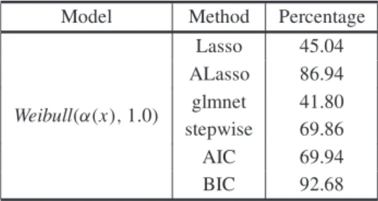
From Table 6 it can be observed that the percentage by which the true model is correctly identi-fied is higher for scenarios that presented larger numbers of covariates (see also Table 3) for all methods. The BIC method is again the best procedure, followed again by ALasso. The AIC, in this scenario, does not present good results, and Lasso is even worse, followed byglmnet.
Table 6– Percentage of correct model selection, Scenario 4.
Model Method Percentage
Weibull(α(x),1.0)
Lasso 45.04 ALasso 86.94 glmnet 41.80 stepwise 69.86 AIC 69.94 BIC 92.68
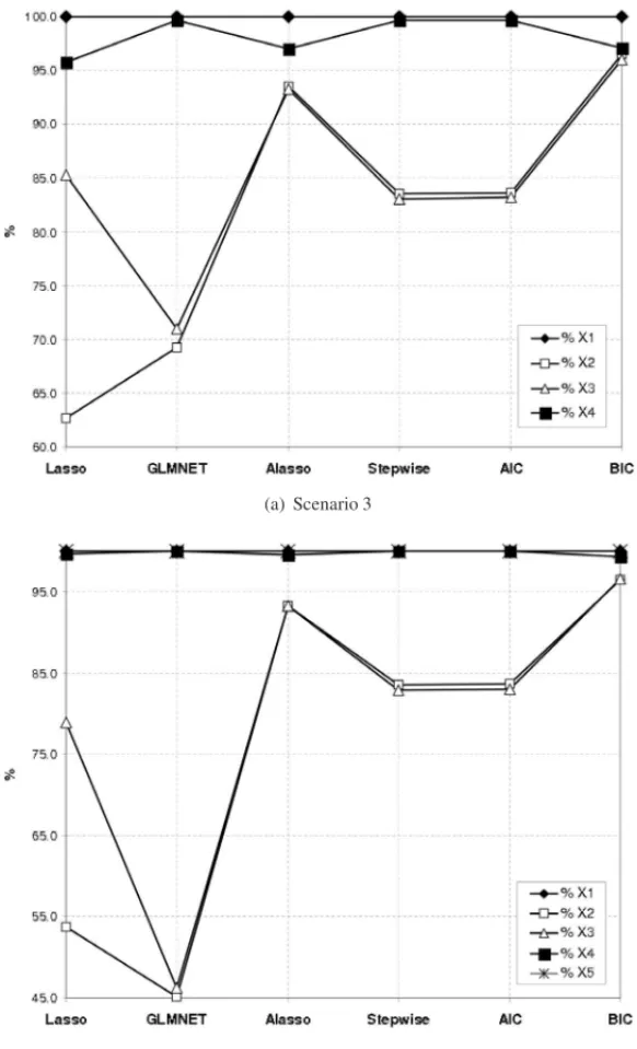
Regarding the performance of Lasso method for selecting each covariate, Figure 6 shows that for scenarios 3 and 4 the Lasso andglmnetmethods frequently select the true covariates. Never-theless, it usually includes some additional covariates which compromises its capacity to detect only the true covariates. BIC and ALasso performances are very close but BIC provides the best results.
In order to illustrate the use of the proposed Lasso and ALasso algorithms, and the other variable selection methods, discussed previously, they are presented below to analyze the data set reported in Fleming and Harrington [22].
6 EXAMPLE: THE PBC DATA SET
(a) Scenario 3
(b) Scenario 4
Figure 6– Percentage of correct covariate selection for scenarios 3 and 4.
the number of days between registration and the earliest death by cirrhosis of liver. Data related to patients submitted to liver transplantation or that died by other causes except cirrhosis were considered as censored observations. The covariates considered in the study are:
X3: Sex, 0 = male 1=female; X4: Presence of ascites; X5: Presence of hepatomegaly; X6: Presence of spiders; X7: Presence of edema; X8: Serum bilirubin, in mg/dl; X9: Serum Cholesterol, in mg/dl; X10:Albumin, in gm/dl;
X11: Urine cupper, inµg/day; X12: Alkaline phosphatase, in U/liter; X13: SGOT, in U/ml;
X14: Triglycerides, in mg/dl; X15: Platelet count;
X16: Prothombin time, in seconds;
X17: Histologic stage of disease, graded 1, 2, 3 or 4.
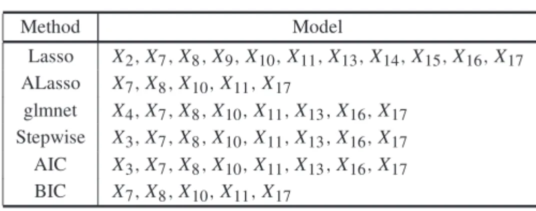
The most parsimonious models selected to describe the behavior ofTprovided by each procedure are given in Table 7.
Table 7– Selected models for each method – PBC data set.
Method Model
Lasso X2,X7,X8,X9,X10,X11,X13,X14,X15,X16,X17 ALasso X7,X8,X10,X11,X17
glmnet X4,X7,X8,X10,X11,X13,X16,X17 Stepwise X3,X7,X8,X10,X11,X13,X16,X17 AIC X3,X7,X8,X10,X11,X13,X16,X17 BIC X7,X8,X10,X11,X17
Notice from Table 7 that all procedures indicate that variables X7,X8,X10,X11andX17should be in the model. Comparing the models obtained using the ALasso and BIC procedures, they are exactly the same. However, the computing cost related to the BIC approach is 3.3 times higher than the ALasso approach. Since there are 17 variables, the BIC approach tested 131,071 possible combinations. The ALasso algorithm used a maximum number of steps equal to 40,000.
Table 8 shows estimates of the coefficients and standard deviations in parentheses. Standard devi-ations were estimated by fitting the regular Cox model with the selected covariates, as suggested by Tibshirani [12, 15].
Table 8– Coefficients’ estimates and standard deviations for PBC data set.
Variables Full Model AIC, stepwise LASSO ALASSO, BIC GLMNET
X1 –0.18 (0.20) — — — —
X2 0.01 (0.01) — 0.02 (0.01) — —
X3 –0.46 (0.29) –0.46 (0.26) — — —
X4 0.11 (0.37) — — — 0.08 (0.34)
X5 0.08 (0.23) — — — —
X6 0.01 (0.23) — — — —
X7 0.97 (0.37) 0.78 (0.34) 0.89 (0.36) 0.81 (0.32) 0.67 (0.33)
X8 0.08 (0.02) 0.09 (0.02) 0.07 (0.02) 0.10 (0.02) 0.08 (0.02)
X9 4e-4 (4e-4) — 5e-4 (4e-4) — —
X10 –0.72 (0.29) –0.74 (0.25) –0.63 (0.26) –0.70 (0.25) –0.65 (0.27)
X11 3e-3 (1e-3) 3e-3 (1e-3) 4e-3 (1e-3) 4e-3 (1e-3) 4e-3 (1e-3)
X12 -3e-5 (4e-5) — — — —
X13 3e-3 (2e-3) 3e-3 (2e-3) 3e-3 (2e-3) — 3e-3 (2e-3)
X14 –1e-3 (1e-3) — –6e-4 (1e-3) — —
X16 0.16 (0.11) 0.17 (0.10) 0.16 (0.10) — 0.17 (0.10)
X17 0.50 (0.16) 0.51 (0.13) 0.51 (0.14) 0.52 (0.13) 0.50 (0.14)
7 CASE STUDY: A BRAZILIAN TELEPHONE COMPANY DATA SET
A certain Brazilian telephone company used to have a small number of clients owing their bills. However, after a huge expansion of the company, the number of unpaid bills grew very fast leading it to change its policies for accepting a new client. In order to establish rules that are flexible enough to still allow the company to grow and also strict enough to avoid a large number of unpaid bills, a study was carried out to identify, among the variables related to the clients characteristics, the ones that could explain their tendency to be in debt with the company. A sample of 530 clients was randomly selected from the company data base. The response variable is the number of days between registration in the data base and its first unpaid bill. The percentage of failures is 60%. The covariates considered in the study are:
X1: Client local calls restriction (1 yes; 0 no); X2: Client budget restriction (1 yes; 0 no); X3: Client general calls restriction (1 yes; 0 no); X4: Number of payment parcels made to the company;
X5: Client has more than one unpaid bill in the past (1 yes; 0 no); X6: Client has automatic debt in his bank account (1 yes; 0 no); X7: Client has not paid the first bill (1 yes; 0 no);
X8: Client has more products from the company (1 yes; 0 no).
since the curve reaches zero which means that all clients in data base eventually stopped paying their bills. Thus, since the response variable is the number of days between registration in the data base and the first unpaid bill, eventually, most of the customers will pay at least one bill after due date. This is the most likely situation because only 12.3% of the clients in the database had automatic debit in banking account, known as an unpopular choice among Brazilians which do prefer mail bills.
In addition, since the date at which the customer enters the database might be different from the due date of the bill, and different customers can choose different due dates, it is natural to use the number of days as the measure of time for the Cox model. By using a daily basis unit as the measure of time and a follow-up around 10,000 days the standard Cox-model can be used in a continuous scale.
0 2000 4000 6000 8000 10000
0.0
0.2
0.4
0.6
0.8
1.0
Survival time (in days)
s(t)
Figure 7– Kaplan-Meier curve for the analysis of the Brazilian Telephone Company data set.
Models selected by the proposed methods are presented in Table 9. Results show that ALasso, stepwise, AIC and BIC selected exactly the same model with three covariates: X1,X5andX6. The Lasso solution included the covariate X4which is not statistically significant, as shown in Table 10. Theglmnetsolution has the greatest number of variables.
higher (e0.57) as compared to clients with no previous unpaid bills. Finally, clients with payments automatically debited from their bank accounts have hazard rates of 42% smaller (1−e−0.54) as compared to clients with no automatic debits.
Table 9– Selected models for each method – Telephone data set.
Method Model Lasso X1,X4,X5,X6 ALasso X1,X5,X6
glmnet X1,X3,X5,X6,X7,X8 Stepwise X1,X5,X6
AIC X1,X5,X6 BIC X1,X5,X6
Table 10– Coefficients’ estimates and standard deviations for Telephone data set.
Variables Full Model LASSO GLMNET others
X1 0.62 (0.18) 0.63 (0.18) 0.61 (0.18) 0.64 (0.17)
X2 0.10 (0.28) — — —
X3 0.14 (0.35) — 0.09 (0.32) —
X4 –0.03 (0.10) 0.01 (0.08) — —
X5 0.54 (0.23) 0.56 (0.23) 0.51 (0.22) 0.57 (0.21)
X6 –0.52 (0.17) –0.53 (0.17) –0.52 (0.17) –0.54 (0.17)
X7 0.52 (0.42) — 0.49 (0.42) —
X8 –0.10 (0.21) — -0.10 (0.21) —
8 DISCUSSION AND CONCLUSION
In this paper, new implementations of the Lasso and ALasso methods for variables selection in the Cox model were proposed to address the problem of selecting the profile of in debt clients of a Brazilian Telephone Company. Their performances were compared with some standard tech-niques for variable selection, such as stepwise, BIC and AIC, through a Monte Carlo study.
From the Monte Carlo study it could be concluded that the BIC method achieved the best perfor-mance followed by the ALasso. Lasso, in general, presented the worst perforperfor-mance. All methods had their performances affected by the sample sizes, the presence of censoring observations as well as by the characteristic of failure rate function.
For the Brazilian Telephone Company data set, the ALasso, stepwise, AIC and BIC selected the same model with three covariates. Since BIC and ALasso methods were pointed out as the best ones in the simulation study, the company should use the model as the reference to define future policies.
Although the BIC method achieved the best results in the simulation study, it tests all possible combinations of the covariates. Consequenly, as the number of covariates increases the comput-ing time gets very high. Therefore, the BIC method is unsuitable when the number of covariates is large. When compare to the BIC method, the ALasso approach is computationally affordable and provides similar results than BIC. The simulation study suggest that the difference between BIC and ALasso is that the latter usually includes some additional covariates. This analysis suggests that combing BIC and ALasso methods would provide better results than just applying BIC or ALasso alone. Therefore, we suggest the following approach: first apply ALasso method to select the initial set of covariates and then run BIC algorithm using the reduced number of covariates selected by the ALasso method.
Discussions highlight that the proposed and original Lasso and ALasso algorithms have distinct features as their main advantages. The original algorithms have the ability to generate arbitrary solutions and our approach is insensitive to numerical problems. Further work aims at combining both approaches by first reaching a reasonable estimator using the original approach and then providing a fine grid of solutions using the proposed approach, taking the best of each algorithm. This is an interesting topic for future research.
ACKNOWLEDGEMENTS
The authors thank CNPq, CAPES and FAPEMIG for financial support.
REFERENCES
[1] COXDR. 1972. Regression Models for Life Tables (with discussion).Journal of the Royal Statistical Society, B,34: 187–220.
[2] COXDR. 1975. Partial Likelihood.Biometrika,62: 269–276.
[3] COXDR & OAKESD. 1984.Analysis of Survival Data, London, Chapman and Hall.
[4] KALBFLEISHJD & PRENTICERL. 2002.The Statistical Analysis of Failure Time Data, New York, Wiley.
[5] LAWLESSJF. 2002.Statistical Models and Methods for Lifetime Data, New York, Wiley.
[6] DRAPERNR & SMITHH. 1998.Applied Regression Analysis, New York, Wiley.
[7] GONCALVESLB & MACRINILR. 2011.Pesquisa Operacional,31(3): 499–519.
[8] GEORGEEI & MCCULLOCHRE. 1995. Two Approaches to Bayesian Model Selection with Ap-plications.In Bayesian Statistics and Econometrics: Essays in Honor of Arnold Zellner(Edited by BERRYD, CHALONERK & GEWEKEJ): 339–348, New York, Wiley.
[9] GEORGE EI & MCCULLOCH RE. 1997. Approaches for Bayesian Variable Selection.Statistica Sinica,7: 339–373.
[10] FARAGGID & SIMONR. 1998. Bayesian Variable Selection Method for Censored Survival Data.
Biometrics,54: 1475–1485.
[12] TIBSHIRANIRJ. 1996. Regression Shrinkage via the Lasso.Journal of the Royal Statistical Society, Series B (Methodological),58(1): 267–288.
[13] KNIGHTK & FUW. 2000. Asymptotics for lasso-type estimators.Annals of Statistics,28: 1356– 1378.
[14] FOSTERSD, VERBYLAAP & PITCHFORDWS. 2008. A random model approach for the Lasso.
Computational Statistics,23: 217–233.
[15] TIBSHIRANIRJ. 1996. The Lasso method for variable selection in the COX model.Statistics in Medicine,16: 385–395.
[16] ZHANGHH & LUW. 2007. Adaptive Lasso for Cox’s proportional hazards model.Biometrika,94: 691–703.
[17] ZOUH. 2008. A note on path-based variable selection in the penalized proportional hazards model.
Biometrika,95: 241–247.
[18] FRIEDMANJ, HASTIE T & TIBSHIRANI R. 2010. Regularization Paths for Generalized Linear Models via Coordinate Descent.Journal of Statistical Software,33(1).
[19] FRIEDMANJ, HASTIET, HOEFLINGH & TIBSHIRANIR. 2007. Pathwise Coordinate Optimization.
The Annals of Applied Statistics,2(1): 302–332.
[20] SIMONN, FRIEDMANJ, HASTIET & TIBSHIRANIR. 2011. Regularization Paths for Cox’s Pro-portional Hazards Model via Coordinate Descent.Journal of Statistical Software,39(5).
[21] TIBSHIRANIRJ, FRIEDMANJH & HASTIETJ. 2003.The Elements of Statistical Learning: Data Mining, Inference, and Prediction, Springer.
[22] FLEMINGTR & HARRINGTONDP. 1991.Counting Processes and Survival Analysis, New York, Wiley.
[23] MARQUARDTDW & SNEE RD. 1975. Ridge Regression in Practice.The American Statistician,
29(1): 3–20.
[24] LENGC, LINY & WAHBAG. 2004. A Note on the Lasso and Related Procedures in Model Selection.
Technical Report no. 1091r.
[25] LAWSONC & HANSENR. 1974.Solving Least Squares Problems, Englewood Cliffs: prentice Hall.
[26] FUW. 1998. Penalized regression: the bridge versus the lasso.Journal of Computational and Graph-ical Statistics,7: 397–416.
[27] COLLETTD. 2003.Modelling Survival Data in Medical Research, London, Chapman and Hall.