A Work Project, presented as part of the requirements for the Award of a Masters Degree in Finance from the Faculdade de Economia da Universidade Nova de Lisboa
“The Fitting of the German Yield Curve: A Dynamic Approach using
Latent, Macroeconomic and Stock Market Variables”
José Pedro Abreu Almeida – Masters Number 172
A Project carried out on the Fixed Income course, with the supervision of: Prof. Paulo Leiria
Page 2 of 28
Abstract
The purpose of this Work Project is to build a yield curve model for the German Government yield curve containing latent variables (Level, Slope and Curvature), macroeconomic variables (German IFO and Inflation Rate) and a stock market variable (German Stock Index DAX), while studying the yield curve dynamics.
The model incorporates the Nelson and Siegel (1987) factor model under a State-Space framework and the estimation results provided a good fitting of the historical yield curve. Additionally, after doing a Variance Decomposition analysis, this project proves the existence of an interaction between the yield curve and the German Macroeconomy/Stock Market.
Keywords: Yield Curve, State-Space Model, Macroeconomy, Stock Market.
Acknowledgements: I thank Professor Paulo Rodrigues, from Universidade Nova de Lisboa, for providing help regarding Econometric research. I also thank Professor Raul Guerreiro, from Universidade do Algarve, for helping with the simulation of the state-space models here presented.
Page 3 of 28
1. Introduction
The term structure of the interest rates (yield curve) is one of the most important financial instruments, as it is used for fixed income securities valuation, for the development of no-arbitrage models, and it is also a good proxy of future spot and inflation rates.
The purpose of this Work Project is to build a model to fit the German Government yield curve. The choice of this yield curve is mainly due to the availability of data. However, instead of using a model containing only latent factors, this Work Project will use a model that can incorporate known variables, namely macroeconomic and stock market variables. In Section 2 of this project, a brief literature review of the existing fitting models will be presented.
This Work Project will follow the Diebold, Rudebusch and Aruoba (2004) framework to build and analyze the dynamics of the German Government yield curve. It uses the traditional Nelson and Siegel (1987) term structure model under a state-space framework that allows the incorporation of macroeconomic and stock market variables. Since, the Diebold, Rudebusch and Aruoba (2004) model is an improvement over Diebold and Li (2002), it will be mandatory to use Diebold and Li (2002)’s approach to obtain some of the necessary inputs of the model. All of these procedures will be described in detail in Section 3.
The main reason for choosing this model is that it allows the incorporation of known factors, meaning exogenous variables. Moreover, since one of this project purposes is to describe the dynamics of the yield curve, the literature suggests that a factor model was more appropriate to use.
Page 4 of 28 Section 4 will be dedicated to the Data, namely the gathering process and some of the Data descriptive statistics. During the analysis (Section 5), the yield data will be used according to Diebold and Li (2002)’s approach to analyze the dynamics of the estimated Level, Slope and Curvature factors (Section 5.1).
In Section 5.2, the state-space framework will be used to estimate a “Latent Model”, under the Diebold, Rudebusch and Aruoba (2004) assumptions, and to obtain the dynamics of the latent factors. Subsequently, and in the same section, an “Extended Model” containing the macroeconomic variables will be built and estimated. A comparison between these two models will be made, while determining how the yield curve dynamics are affected by the latent (unobserved) factors and the macro/stock market (observed) factors. In other words, in addition to the fitting of the yield curve, this Work Project’s purpose is to see if, and how, the Macroeconomy and Stock Market influence the yield curve dynamics.
In section 6, conclusions and final remarks will be presented.
2. Brief Literature Review
One of the main characteristics of the fitting models should be their smoothness and flexibility; as Jabbour and Mansi (2002) put it, “Smoothness in this case is defined as the ability of the model to remove noise from the data and to accommodate various bends in the term structure”.
We may have Parametric or Non-Parametric models that estimate the yield curve. Parametric models assume a functional form of the yield curve, with determined parameters, like “level”, “slope” and “curvature” from Nelson and Siegel (1987), while the Non-Parametric models use polynomial functions that are linked through a number
Page 5 of 28 of “knot points”. The main advantages of Parametric Models are the avoidance of problems regarding the selection of “optimal knot points” and they also force “the interpolated (forward) rate at the long end of the curve to a horizontal asymptote” (Jabbour and Mansi (2002)).
Using Nelson and Siegel (1987), a dynamic model was developed by Diebold and Li (2002), where they “distill the entire yield curve, period-by-period, into a three-dimensional parameter that evolves dynamically” and interpret these time-varying parameters as factors.
Additionally, there are models which adopt the equilibrium approach or the no-arbitrage approach. The no-no-arbitrage approach wants to assure that the yield curve is fitted such that there are no arbitrage opportunities, while, as in Rotondi (2005), “the equilibrium approach focuses on modeling the dynamics of the instantaneous rate typically using affine models”. Some of the most famous equilibrium approach models are the Vasicek (1997) and Cox, Ingersoll and Ross (1985) and no-arbitrage models are Duffie and Kan (1996).
All of these models capture the dynamics of the yield curve through linear functions of latent factors, but they fail to identify the shocks to the yield curve from other outside sources, like macroeconomic factors.
Arturo Estrella (2005), in his paper, gives a good insight on the existing evidence regarding the relationship between the “term-spread” and real economic activity; “various spreads between long and short-term rates tend to be low at the start of recessions”. The difference between the ten-year and three-month Treasury rates became a rule of thumb when predicting future recessions, as well as yield curve inversions. Estrella and Mishkin (1998) compare “the term structure as a predictor of
Page 6 of 28 recessions with a large number of alternative indicators and find that it is among the best in tests of statistical significance”.
A large group of the studies point, however, that the predictability is highly related to monetary policy credibility. It is common sense that “expected future short-term rates are important deshort-terminants of current long-short-term rates” (Arturo Estrella (2005)). A tighter monetary policy will have a negative impact on the economy and may flatten the yield curve, but “monetary policy is not likely to be the single determinant of the predictive power” of the yield curve.
The last two decades have shown a huge development of yield curve models containing other macroeconomic variables, namely the Nelson and Siegel and affine no-arbitrage dynamic latent factor models. On one hand, Diebold, Rudebusch and Aruoba (2004) incorporate the dynamic Nelson and Siegel factor model of Diebold and Li (2002) into a State-Space framework using a Vector AutoRegression. Additionally, they incorporate real activity, monetary policy instrument and inflation together with the three latent factors (level, slope and curvature). On the other hand, Ang and Piazzesi (2001) developed “A No-arbitrage Vector Auto Regression of Term Structure Dynamics with Macroeconomic and Latent Variables”, which is an affine model imposing no-arbitrage and the independency between policy interest rate and inflation, as well as real economic activity.
Finally, Rudebusch and Wu (2003) incorporate inflation and capacity utilization along with latent factors in a model that allows bi-directional feedback between macroeconomic variables and latent factors. Therefore, like stated in Arturo Estrella (2005), the yield curve may be a predictor of the future economic activity, but “in
Page 7 of 28
L
S
e
C
e
e
y
t t t1
t1
e
e
e
y
1 21
31
principle there could be influences in the opposite direction, from economic activity to the yield curve”.
3. Methodology
As said before, Diebold, Rudebusch and Aruoba (DRA (2004)) framework will be used to do the fitting and analysis of the dynamics of the German Government yield curve. This model follows some of the assumptions of Diebold and Li (DL (2002)), as they interpret the Nelson and Siegel (Equation (1)) “in a dynamic fashion as a latent factor model in which β1, β2 and β3 are time-varying level, slope and curvature factors
and the terms that multiply these factors are the factor loadings” (Equation (2)).
(1)
(2)
Where β1, β2 and β3 and are parameters and, on the Equation (2), Lt, St and Ct are time
varying β1t, β2t and β3t. The parameter is the decay parameter of the Nelson and Siegel
function; “small values of produce slow decay and can better fit the curve at long maturities, while large values of, produce fast decay and can better fit the curve at short maturities”.
In order to forecast the Nelson and Siegel Level, Slope and Curvature, DL(2002) estimate β1, β2 and β3 through Ordinary Least Squares for each available period, and,
Page 8 of 28 t t t
Y
) 1 3 ( ) 1 3 ( 1 1 1 ) 3 3 ( 33 32 31 23 22 21 13 12 11 ) 1 3 ( ) 1 3 ((
)
)
(
)
(
x t t t x t t t x x C S L x t t tC
S
L
C
S
L
a
a
a
a
a
a
a
a
a
C
S
L
t t t t
1
( 1) 2 2 1 1 ) 1 3 ( ) 3 ( 2 2 1 1 ) 1 ( 2 1 1 1 1 1 1 1 1 1 1 2 2 2 1 1 1 Nx N N x t t t Nx N N Nx N t t t C S L e e e e e e e e e y y y N N N (2004) adopted the following State-Space model to estimate and forecast the same factors, while assuming a VAR (1) of the dynamics of Lt, St and Ct:
- (3) Transition Equation
(3)
- (4)Measurement Equation
(4)
Where “τ” stands for maturity in months Vector notation:
(5)
(6)
The transition equation (3) states the dynamics of the state vector; as we can see, t
follows a First-Order Autoregressive Process, maintaining the same assumption as in DL (2002). This is in line with the statement that “ARMA state vector dynamics of any order may be readily accommodated in state-space form” DRA (2004). Vector t is the disturbance vector of the transition equation.
Page 9 of 28
) 12 ( ) 3 3 ( ) 1 ( ) 1 3 (0
0
,
0
0
~
Nx x Nx x t tH
Q
WN
The measurement equation (4) represents the common Nelson and Siegel structure: Yt is the set of historical yield curves along the sample period and they are
related to the three latent factors, vectort, whose behavior is described by the measurement equation. Matrix is the matrix containing the loadings of the unobserved factors for the N given maturities. Similarly to the transition equation t is the vector of the disturbances of the measurement equation.
Together, these two equations form a state-space model and, as an assumption, “the white-noise transition and measurement disturbances must be orthogonal to each other and to the initial state” DRA (2004):
(7)
(8)
During my analysis, like in DRA (2004), the H matrix will be assumed as diagonal, implying that the errors of the different maturities are uncorrelated. Nevertheless, Q matrix will be non-diagonal to allow shocks to the three term structure factors to be correlated.
This state-space model is an improvement to the DL (2002) model, because it allows the estimation of all parameters simultaneously via the Kalman Filter, delivering “maximum-likelihood estimates and optimal filtered and smoothed estimates of the underlying factors” DRA (2004). Moreover, in just one procedure, it is possible to obtain the estimated factors for all the data periods. Nevertheless, the analysis (Section 5) will begin by the estimation of the latent factor series, as in DL (2002), (Section 5.1), because they are required for the state-space model specification (Section 5.2).
'
0 0 ' 0 0 t t E E
Page 10 of 28
4. The Data
4.1. Yield Data
Despite being a state-space approach, the Nelson and Siegel (1987) model will still require historical data on the German yield curve. The German historical yield curves were obtained, through Bloomberg, using Bund STRIPS of the following maturities: 3 Months (3M), 6 Months (6M), 1 Year (12M), 2 Years (24M), 3 Years (36M), 4 Years (48M), 5 Years (60M), 6 Years (72M), 7 Years (84M), 8 Years (96M), 9 Years (108M) and 10 Years (120M).
The Bund STRIPS are “zero-coupon securities and, as a result, provide direct observation of spot rates” (Jabbour and Mansi (2002)). Additionally, STRIPS are available for a large number of maturities and fungible. One inconvenient for using the STRIPS is that they may have liquidity problems due to limited supply, which lead to the exclusion of the 15 Years and 30 Years maturities from my sample.
All of these spot interest rates, which range from March 1995 to 2010, were obtained on a Monthly Basis collected at the end of the month and are bid-ask averages. (Bloomberg tickers are GETΒ1, GETΒ2 and GDBR1-10). Table 1 contains some of their descriptive statistics.
Page 11 of 28 4.2. Macroeconomic and Stock Market Data
The exogenous variables, collected from Bloomberg, are the German IFO, the German Inflation Rate and the German Stock Index DAX. The first two are important macroeconomic fundamentals and the last one represents the stock markets.
Since the Gross Domestic Product has a quarterly basis, a monthly proxy could improve the estimation. The German IFO represents German Business Expectations and is it commonly used as a proxy for Gross Domestic Product growth (the correlation between the GRIFPEX (German IFO) and the growth rates of GRGDEGDP Index (German GDP), using quarterly data from 1995-2009, is 0.65). The German Inflation Index used to compute the monthly inflation rate is the Consumers Price Index using the 2005 prices. The monthly inflation rate will be called “INFL”.
Unlike the other variables, the DAX data from March 1995 until 2010 was obtained on a daily basis and afterwards a monthly average was computed. This had the purpose of avoiding price miss-specification at the end of the month due to “behavioral finance” issues. The monthly average growth rate of the DAX is the variable that will be used during my project and will be called “DAX”. Table 2 contains the descriptive statistics of the chosen variables.
Page 12 of 28
5. Analysis
5.1. The Nelson and Siegel Dynamic Framework
Being a factor model, the Nelson and Siegel (1987) follows the “parsimony principle” and, according to Diebold, Piazzesi and Rudebusch (2005), it is “the broad insight that imposing restrictions – even those that are false and may deteriorate in-sample fit – often helps both to avoid data mining and to produce good forecasting models”.
If we look at the loadings of the model, at a certain fixed , on β1 loading is
always 1 and the one on β2 starts at 1 and converges to 0. Finally, the loading on β3
starts at 0 and, after increasing, begins to converge to 0 again. This behavior of the loadings are displayed in Figure 1 using =0.0609 as used in DL (2002). As recommended by DL (2002),will be fixed at 0.0609 for all the remaining work.
Figure 1 – Nelson and Siegel (1987) Factor Loading, with constant =0.0609. Subsequently and, due to the factor loadings behavior, one of the most interesting points of this model is also the possibility of interpreting its latent factors; β1
is commonly referred as the long-term factor, β2 the short-term factor and β3 the
Page 13 of 28 level, slope and curvature of the yield curve. As in DL 2002, “Level” is defined as the
M
yt 120 , “Slope” as yt
120M
yt
3M and “Curvature” as
M
y
M
y
Myt 24 t 120 t 3
2 . Level, Slope and Curvature were obtained, using the historical yield curves, and some of their statistics are presented in Table 3. Like in DL 2002, the factors are not highly correlated; corr(level, slope)= -0,32, corr(level, curvature)= 0,23 and corr(slope, curvature)= -0,57.
Table 3 – Level, Slope and Curvature Descriptive Statistics.
From a dynamic perspective, DL (2002) showed that the Nelson and Siegel model may be rewritten as in Equation (2). Therefore, using the Ordinary Least Squares for all the data periods it is possible to obtain a series of 181 β1, β2 and β3. Table 4
contains the descriptive statistics of these series.
Page 14 of 28 In order to assess the quality of the German yield curve fit, using the dynamic Nelson and Siegel model, Figure 2 contains the plot of the average actual yield curve along with the average fitted yield curve, which are very close to each other.
Figure 2 – Actual Average Yield Curve versus Average Fitted Yield Curve.
Additionally, it is useful to compare the estimated Level, Slope and Curvature (β1, β2 and β3) with the actual Level, Slope and Curvature from the historical yield
curves Figures 3, 4 and 5); an almost perfect match is visible.
Page 15 of 28
Figure 4 – Estimated -B2 versus Historical “Slope” (as in DL 2002).
Figure 5 – Estimated 0.3*B3 versus Historical “Curvature” (as in DL 2002).
Finally, the correlations between them made me conclude that the estimates of β1, β2 and β3 are good proxies of Level, Slope and Curvature factors for the German
Yield Curve; corr(β1, level)=0.946, corr(β2 , slope)=-0.99, corr(β3, curvature)=0.99.
5.2. Fitting the Yield Curve using a State Space Approach
The previous section explained the dynamics of the Nelson and Siegel model and the interpretation of the latent factors. The previously estimated latent factors (β1, β2
Page 16 of 28 ) 1 3 ( ) 1 3 ( 1 1 1 ) 3 3 ( 33 32 31 23 22 21 13 12 11 ) 1 3 ( ) 1 3 ( ( ) ) ( ) ( x t t t x t t t x x C S L x t t t C S L C S L a a a a a a a a a C S L ) 12 12 ( ) 3 3 ( ) 1 12 ( ) 1 3 ( 0 0 , 0 0 ~ x x x x t t H Q WN t t t t 1 t t t Y (121) 2 1 ) 1 3 ( ) 3 12 ( 0.0609 120 0.0609 120 0.0609 120 0.0609 6 0.0609 6 0.0609 6 0.0609 3 0.0609 3 0.0609 3 ) 1 12 ( 120 6 3 0.0609 120 1 0.0609 120 1 1 0.0609 6 1 0.0609 6 1 1 0.0609 3 1 0.0609 3 1 1 120 6 3 x N x t t t x x t t t C S L e e e e e e e e e y y y
and β3) will also be used under the context of the DRA (2004) state-space approach,
which consists of this new section.
Two state-space models will be built. The first one will estimate the yield curve using only the latent factors and will be followed by an extended version containing the macroeconomic variables (IFO and INFL) as well as the stock market variable (DAX).
5.2.1. Latent Factors Model Specification (“Latent Model”)
Using Equations (3) and (4), it is possible to build the following state-space model adapted to all my assumptions:
Transition Equation: (9) or Measurement Equation: (10) or Error Distribution: (11)
On the measurement equation (10), vector Yt is the dependant variable
Page 17 of 28 72, 84, 96, 108 and 120 months. Matrix contains the loadings related to the yield curve factors “Level”, “Slope” and “Curvature” (vector βt), where equals 0.0609.
Overall, a total of 30 parameters must be estimated: vector μt contains 3
parameters to estimate, the transition matrix ɸ has 9 parameters to be estimated, matrix Q has 6 parameters to be estimated (3 variances and 6 covariances) and matrix H has 12 variances to be estimated.
Before starting the estimation, it is necessary to compute some start up parameters. Therefore, matrix ɸ is initialized as the coefficient matrix of an Unrestricted VAR(1) between the time varying β1, β2, and β3 from Section 5. Vector μt is the
mean-vector of the same factors. Finally, the initial state-mean-vector and variances/covariances are computed through a diffuse maximum likelihood process (Harvey (1989)).
The estimation of the optimal yields and latent factors (state-vector βt) is made
through a multivariate Kalman Filter, using the Broyden, Fletcher, Goldfarb and Shanno (BFGS) technique. Matrices Q, H and ɸ parameters were obtained with a non-linear parameter search with maximum likelihood function.
5.2.2. Extended Latent Factors Model (“Extended Model”)
The Dynamic Nelson and Siegel model under state-space framework allows the inclusion of exogenous variables, which was not possible using the DL (2002). Consequently, together with the usual latent factors β1, β2, and β3, the following model
uses the IFO, INFL and DAX historical values in order to estimate the optimal yield predictions.
Page 18 of 28 t t t t 1 t t t Y ) 1 6 ( ) 1 6 ( 1 1 1 1 1 1 ) 6 6 ( 66 65 64 63 62 61 56 55 54 53 52 51 46 45 44 43 42 41 36 35 34 33 32 31 26 25 24 23 22 21 16 15 14 13 12 11 ) 1 6 ( ) 1 6 ( ( ) ) ( ) ( ) ( ) ( ) ( x t t t t t t x t t t t t t x x DAX INFL IFO C S L x t t t t t t DAX INFL IFO C S L DAX INFL IFO C S L a a a a a a a a a a a a a a a a a a a a a a a a a a a a a a a a a a a a DAX INFL IFO C S L (121) 2 1 ) 1 6 ( ) 6 12 ( 0.0609 120 0.0609 120 0.0609 120 0.0609 6 0.0609 6 0.0609 6 0.0609 3 0.0609 3 0.0609 3 ) 1 12 ( 120 6 3 0 0 0 0.0609 120 1 0.0609 120 1 1 0 0 0 0.0609 6 1 0.0609 6 1 1 0 0 0 0.0609 3 1 0.0609 3 1 1 120 6 3 x N x t t t t t t x x t t t DAX INFL IFO C S L e e e e e e e e e y y y ) 12 12 ( ) 6 6 ( ) 1 12 ( ) 1 6 ( 0 0 , 0 0 ~ x x x x t t H Q WN Transition Equation: (12) or Measurement Equation: (13) or Error Distribution: (14)
As we can see, the structure of the model remains unchanged, but some of the vectors/matrices have now increased dimensions. On the measurement equation (13), matrix is now 12x6, because its associated state-vector is now 6x1. Notice that, “the three rightmost columns contain only zeros, so that the yields still load only on the yield curve factors” (DRA 2004).
In this extended model, a total of 75 parameters must be estimated: vector μt
contains 6 parameters to estimate, the transition matrix ɸ has 36 parameters to be estimated, matrix Q has 21 parameters to be estimated (6 variances and 15 covariances) and matrix H has 12 variances to be estimated.
Page 19 of 28 The initialization and estimation procedures are the same as in Section 6.1, with the exception of the initial matrix ɸ, which is now the coefficient matrix of the Unrestricted VAR(1) of estimated β1, β2, β3 (from Section 5) and the additional IFO,
INFL and DAX historical values.
5.2.3. Estimation Results: Assessing the Fit
The two previous models were used to obtain the optimal yield curve prediction along the period between March 1995 and 2010. While the Latent Model only estimates the time series of β1, β2, β3, the Extended Model also estimates the time series of IFO,
INFL and DAX. Regarding the parameter estimation, the final values of vector μt ,
matrices ɸ, Q and H, for both models, are presented in Appendix 1 and 2.
In order to assess the fit of the models in relation to the historical yield curves, the measurement errors were computed as 𝑦𝑡 𝜏𝑖 − 𝑦 𝑡 𝜏𝑖 (in basis points), for both models, and some statistics regarding the estimated yields were obtained (Table 5).
Table 5 – Statistics of the Estimated Yields from both state-space models (in basis points).
The table above suggests that the quality of the fit is similar in both models and that both of them provide a good fit of the historical yield curves; the quadric mean errors are low as well as the error standard deviation for the different maturities. Finally,
Page 20 of 28 just like in Section 5, the estimated latent factors (β1, β2, β3), from both models, are
plotted along with the actual “Level”, “Slope” and “Curvature” (Figures 6, 7 and 8).
Figure 6 – Estimated B1 versus Historical “Level” (as in DL 2002).
Figure 7 – Estimated -B2 versus Historical “Slope” (as in DL 2002).
Page 21 of 28 Despite small level differences, the behaviors of β1, β2 and β3 series are almost
equal to “Level”, “Slope” and “Curvature”; both models perfectly match the dynamics of the Nelson and Siegel (1987).
It is important to notice that the Extended Model required the estimation of 75 parameters, while the Latent Model required only the estimation of 30 parameters. Even so, the quality of the fit is very similar, meaning that the Extended Model is also a good approach.
5.2.4. Variance Decompositions
In this section, the estimated time series “Level”, “Slope” and “Curvature” (β1,
β2 and β3), from both models, are going to be used in order to explain the forecast
variance of the 3, 60 and 120 Months yields (representing the short, medium and long terms of the yield curve, respectively). For this purpose, a Variance Decomposition analysis will be done for the given yields.
The VAR, as in Stock and Watson (2001), “expresses each variable as a linear function of its own past values, the past values of all other variables being considered and a serially uncorrelated error term”. Subsequently, the Variance Decompositions may be extracted from the VAR; “the forecast error decomposition is the percentage of the variance of the error made in forecasting a variable due to a specific shock at a given horizon” Stock and Watson (2001).
This kind of analysis will show the variation of a certain interest rate is explained by itself, the latent factors and the additional IFO, INFL and DAX variables. Thus, for each maturity (3, 60 and 120 months), there will be two Variance Decomposition analysis: one containing only the estimated latent factors (from the
Page 22 of 28 Latent Model) and another containing estimated latent factors (from the Extended Model) together with IFO, INFL and DAX historical series. The results will tell how are the dynamics of the short, medium and long terms of the yield curve explained by the latent factors and the macro/stock market variables.
Variance Decomposition of 3 Months Interest Rate
Table 6 – V.D. of 3M, up to 60 months forecast, using β1, β2, β3 from Latent Model.
Table 7 – V.D. of 3M, up to 60 months forecast, using β1, β2, β3 from Extended Model.
Under the Latent Model, Table 6, the 3M variation is mostly explained by itself (75%), at the horizon of 5 months, while the remaining variance is explained mostly by β3 (85,5%). However, at longer horizons, its remaining variation is largely explained by
the latent factors β2 (34,5%)and β3 (62,5%). Following Nelson and Siegel (1987), this is
Page 23 of 28 On the Extended Model, Table 7, with an horizon of 60 months, the IFO is the variable that explains the most of 3M variation (32,045), whether β2 and β3 contributions
(11,127 and 13,412) are close to the DAX (12,115). Therefore, in the short-term of the yield curve, the variation of the interest rates is mostly due to the GDP growth (since IFO is a GDP growth proxy). Similarly to all the following Variance Decompositions, the Inflation Rate does not seem to influence the variation of the interest rates, for the selected maturities.
Variance Decomposition of 60 Months Interest Rate
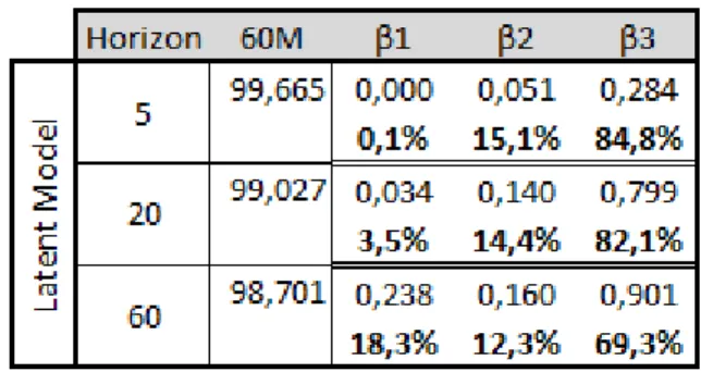
Table 8 – V.D. of 60M, up to 60 months forecast, using β1, β2, β3 from Latent Model.
Table 9 – V.D. of 60M, up to 60 months forecast, using β1, β2, β3 from Extended Model.
From both tables, it is clear that the most part of the 60M variation is due to itself (almost 100% on the Latent Model, Table 8, and more than 55% at the Extended Model, Table 9).
Page 24 of 28 Nevertheless, the remaining variance under the Latent Model is always explained by β3 at a percentage superior to 60%. Being β3 the “Curvature” factor, this
makes sense since the 60M rate is a medium maturity rate.
However, on the Extended Model analysis, it is the IFO, β1, and DAX that are
responsible for the majority of the remaining variance (44,9%, 25,8% and 20,3%, respectively) and it is important to notice that, as the horizon increases, the remaining variance is also increasing.
Variance Decomposition of 120 Months Interest Rate
Table 10 – V.D. of 120M, up to 60 months forecast, using β1, β2, β3 from Latent Model.
Table 11 – V.D. of 120M, up to 60 months forecast, using β1, β2, β3 from Extended Model.
In both models, at the longest horizon, β1 is the one that explains the major part
of the remaining variance (66,2% Latent Model and 35,1% Extended Model), which is understandable since the 120M yield is a long-term yield and β1 represents the long
Page 25 of 28 120M yield than the IFO variable, suggesting that the stock market has more influence over the long term of the yield curve than the GDP.
6. Conclusion
In this Work Project, a yield curve factor model containing latent, macroeconomic (IFO and INFL) and stock market (DAX) variables was specified and estimated, which was called “Extended Model”. Similarly to DRA (2004), this model followed a state-space approach as it allows the incorporation of exogenous variables along with the traditional latent factors of Nelson and Siegel (1987) and, as expected, provided a good fit of the yield curve.
The Variance Decomposition analysis showed that the IFO, INFL and DAX, together, explain the majority of the remaining variance of the yields, for all of the forecasting horizons. This suggests that the yield curve dynamics are better explained by the macroeconomic variables and stock market variables than explained by the latent factors.
From the same analysis, the IFO turned to be the overall most important factor influencing the yield curve dynamics, providing evidence for the strict relationship between the yield curve and GDP growth referred in the literature.
Finally, in the long-term of the yield curve, it is the DAX the variable responsible for the large majority of the yield remaining variation, which is consistent with the relationship between the stock and the bond markets; typically, rising interest rates lead to a decrease in stock prices (and vice-versa). That is why bonds are considered to be an important indicator of the stock market.
Page 26 of 28
References
Andrew Ang, Monika Piazzesi, Min Wei. (2006). “What does the yield curve tell us about GDP growth?” Journal of Econometrics, 131: 359-403.
Andrew Ang. and Monika Piazzezi (2001). “A No-Arbitrage Vector Autoregression of Term Structure Dynamics with Macroeconomic and Latent Variables.” National Bureau of Economic Research.
Arturo Estrella (2005). “The Yield Curve as a Leading Indicator: Frequently Asked Questions”.
Frank J. Fabozzi. (2000) “CFA Bond Markets, Analysis and Strategies”. Prentice Hall International, Inc. 4th Edition.
Francis X. Diebold and Canlin Li (2002). “Forecasting the Term Structure of Government Bond Yields.” Penn Institute of Economic Research.
Francis X. Diebold, Glenn D. Rudebusch and S. Boragan Aruoba. (2004). “The Macroeconomy and the Yield Curve: A Dynamic Latent Factor Approach.” National Bureau of Economic Research.
Francis X. Diebold, Monika Piazzesi and Glenn D. Rudebusch. (2005). “Modeling Bond Yields in Finance and Macroeconomics.” American Economic Review, 95, 415-420.
Francis X. Diebold, Canlin Li, Vivian Z. Yue (2007). “Global Yield Curve Dynamics and Interactions: A Dynamic Nelson-Siegel Approach.”
Page 27 of 28 George M. Jabbour and Sattar A. Mansi (2002). “Yield Curve Smoothing Models of the Term Structure.”
Hisahi Tanizaki (1996). “State-Space Model in Linear Case” – In Nonliniar Filters: Estimation and Applications (Springer-Verlag, 1996). Faculty of Economics, Kobe University
James H. Stock and Mark W. Watson (2001). “Vector Autoregressions.” Journal of Economic Perspectives – Volume 15, Number 4 – Fall 2001 – Pages 101-115.
Miguel Jerez, Sonia Sotoca and José Casals. “E4 A Matalab Toolbox for Time Series Modeling.” Universidad Complutense de Madrid.
Michiel de Pooter (2007). “Examining the Nelson-Siegel Class of Term Structure Models.” Timbergen Institute Discussion Paper.
Nelson, C.R. and Siegel, A.F. (1987). “Parsimonious Modeling of Yield Curves.” Journal of Business 60, 473-489
Siem Jan Koopman, Max I.P. Mallee and Michel van der Wel (2007). “Analysing the Term Structure of Interest Rates using the Dynamic Nelson-Siegel Model with Time-Varying Parameters.” Timbergen Institute Discussion Paper 095/4.
Wei-Choun Yu and Eric Zivot (2010). “Forecasting the Term Structures of Treasury and Corporate Yields: Dynamic Nelson Siegel Models Evaluation.”
Zero Rotondi (2005). “The Macroeconomy and the Yield Curve: A Review of the Literature with Some New Evidence.” Capitalia and University of Ferrara.
Page 28 of 28
Appendix
Matrix H
Matrix Q Matrix ɸ and Vector μ
Appendix 1 – Latent Model final values of Matrix H, Q, Φ and μ.
Matrix H
Matrix Q Matrix ɸ and Vector μ