The Effect of Financial Distress on Earnings Management: An Italian
Case Study
Matteo Zanini
152418007Dissertation written under the supervision of Professor Ricardo Reis
Dissertation submitted in partial fulfilment of requirements for the MSc in Finance, at the Universidade Católica Portuguesa.
The Effect of Financial Distress on Earnings Management: an Italian Case Study Matteo Zanini
Abstract
The present study empirically investigates the relationship between financial distress and earnings management with reference to selected Italian companies, focusing on publicly listed, medium-size entities. Our sample consists of 38 firms, who were polled during the recession period, and afterwards from 2007 to 2017. Our study used discretionary accruals (DA) as a proxy for earnings management, and the cross-sectional modified Jones model has been applied for the estimate thereof. Altman’s Z-score was selected as the measure for financial distress. The study further considers the association between firms in financial distress and earning management changes during the recent global financial crisis. Through a multiple regression analysis, our study finds that highly distressed firms are more likely to engage in earnings management practices that financially sounder counterparts. Size is found to have a significant positive relationship with earnings management, implying that bigger firms are more inclined to accounting manipulation through DA. Profitability, on the other hand, showed negative correlation. The study found evidence of the effect of the financial crisis on this relationship between earnings management and financial distress, showing that distressed firms engage in income-increasing earnings management activities much more extensively during periods of financial crisis. The findings of the study have important implications for investors who want to make better investment decisions, as well as regulators, who are responsible for monitoring financial reporting quality.
Keywords: Earnings management, financial distress, Italy, global financial crisis Sustainable Development Goals (SDGs): 8, 9
The Effect of Financial Distress on Earnings Management: an Italian Case Study Matteo Zanini
Resumo
O presente estudo investiga empiricamente a relação entre as dificuldades financeiras e a gestão dos lucros, com referência a empresas italianas selecionadas, cotadas em bolsa de tamanho médio. A nossa amostra consiste em 38 empresas, que foram sondadas entre 2007 e 2017. O estudo usa acréscimos discricionários como substituto da gestão dos lucros, e o modelo modificado de Jones foi aplicado à estimativa. O Z-score de Altman foi selecionado como medida para as dificuldades financeiras. O estudo considera ainda a associação entre empresas em dificuldades financeiras e modificações na gestão de lucros durante a crise financeira global. Através de uma análise de regressão múltipla, o nosso estudo descobre que empresas em dificuldades financeiras graves têm maior probabilidade de praticarem atos de gestão de lucros do que os seus pares em melhor situação financeira. Compreende-se que o tamanho da empresa tem um impacto positivo significativo na relação com a gestão de lucros: empresas de maior dimensão têm maior probabilidade de manipular a contabilidade através de acréscimos discricionários. A rentabilidade mostra uma correlação negativa. O estudo encontrou provas do efeito da crise financeira nesta relação entre gestão de lucros e dificuldades financeiras, mostrando que empresas em situações financeiras mais delicadas tomam parte em ações de gestão de lucros de forma muito mais intensa em períodos de crise financeira. As conclusões do presente estudo têm implicações importantes para investidores que queiram tomar melhores decisões de investimento, tal como para reguladores, que são responsáveis por monitorizar a qualidade da comunicação financeira.
Palavras-chave: Gestão de lucros, dificuldades financeiras, Itália, crise financeira global Objetivos de Desenvolvimento Sustentável (ODS): 8, 9
Acknowledgments
This dissertation represents the beginning of a journey, rather than an end. A journey that took me to put myself on the line and quit a career in another business field to move toward different and more ambitious career goals.
First, I wish to express my deepest gratitude to my supervisor, Professor Ricardo Reis, for providing guidance, support and feedback throughout this project.
A special thanks to my co-workers Jose Quintella, Ricardo Lages, Rafael Nogueira, Filipe Figueiredo, Angelo Migliorino and Luis Henriques, who have supported me and provided their advice during these intense months.
I would like also to thank all the Católica colleagues and friends, with whom I shared this experience, gained knowledge and became a better person.
Finally, my biggest thanks to my family. Without them, this achievement simply would not have been possible.
Table of Contents
1. Introduction 8
2. Literature Review and development of hypotheses 10
2.1 Literature Review 10
2.2 Earnings Management and Financial Distress: Research Hypotheses 15
3. Research Design and Methodology 17
3.1 Sample description and Data 17
3.2 Measurement of financial distress: Altman’s Z-score 18
3.3 Measurement of Earnings Management 20
3.4 Regression Models and Research Variables 22
4. Empirical results 24
5. Conclusions 31
6. References 32
List of Tables
Table 1. Industry-wide distribution of sample firms based on the industry classification benchmark (ICB)
18
Table 2. Descriptive Statistics and correlation analysis 25
Table 3. Association between discretionary accruals and financial distress 27 Table 4. Association between discretionary accruals and financial distress one year behind 28 Table 5. Impact of the global financial crisis on the association between discretionary
accruals and financial distress
30
Table 6. First regression model - ANOVA results 35
Table 7. Collinearity diagnostics 35
Table 8. Correlations analysis 36
Table 9. Second regression model – ANOVA results 37
Table 10. Model Summary 37
Table 11. Collinearity diagnostics 37
Table 12. Residuals Statistics 38
Table 13. Descriptive statistics 38
Table 14. Third regression model – ANOVA results 39
List of Abbreviations
DA Discretionary Accruals NDA Non-discretionary Accruals
GAAP Generally Accepted Accounting Principles TA Total accruals
OLS Ordinary least square FC Financial crisis
1. Introduction
The objective of the present paper is to investigate and provide further insight on an issue that, especially in this period following a severe financial crisis, has proven to be extremely important from a social and economic point of view: managerial earnings management behaviours of financially distressed firms. Corporate financial distress has long been a major concern not only for firms’ stakeholders, but also for governments that need to take measures to reduce possible systemic risks. Companies inevitably fall into financial distress because of a weakening in their performance and the consequences may be devastating, including bankruptcy filing or acquisition by other firms. Therefore, it becomes crucial for regulators and stakeholders to spot potential warning signs in the management of the firm before the conditions become irreversible. In case of firm bankruptcy, investors and creditors are of course the most directly affected but the impact can also be significant on the overall economic context. When facing financial distress, management has strong incentives to camouflage deteriorating financial indicators and to adopt accounting policies that boost the income of the firm. The necessity to report target earnings, cuts in management bonusses, loss of reputation, continuation in obtaining credit from banks, contractual negotiations and fear of losing their job positions are all probable reasons behind earnings management actions. For listed companies, the reactions from financial markets are traditionally one of the most important arguments behind these decisions and share price is strictly influenced by wide variations in earnings or lower estimates. Earnings manipulation can thus be an effective tool in the hands of managers to smooth out such variations (Barnea, et al., 1976). Empirical evidence, however, does not lead to a definitive conclusion: some authors (Rosner, 2003) predict that ex-post bankrupt firms which did not appear distressed ex-ante, have significantly greater material income-increasing accruals magnitudes than control firms. Conversely, another author (DeAngelo, et al., 1994) documented that managers flatten earnings through negative abnormal accruals and discretionary write-offs, instead of inflating income.
In the present paper, I analysed financial statements from publicly listed Italian companies, exclusively considering the components of the stock market index FTSE Italia Mid Cap as of 31/12/2019. As consistent with previous studies, constituents belonging to finance and banking industries were excluded from the sample since their financial statements respond to different criteria and their accounting measures are not comparable with their nonfinancial counterparties, especially in terms of leverage. For similar reasons, companies from the real estate and insurance industries were omitted.
FTSE Italia Mid Cap companies have been chosen for the sample due to a number of reasons. My personal background and financial knowledge of the local market played a role. Additionally, the mid-cap segment represents, in our view, the best scenario to analyse the causal relationship in question, since it includes all kinds of possible companies, both in good shape and in distressed condition. With the purpose of assessing the quality of earnings and gauging whether distressed companies engage in earnings manipulation practices more than ‘healthy companies’ the classic version of the Modified Jones model has been used.
The motivations behind this study are multiple. Firstly, based on data in our possession, there has been an increasing trend of defaults in Italy in the period subsequent to the most recent financial crisis. Secondly, according to the studies presented in the literature review, the relationship between the level of distress and earnings management still appears to be inconclusive. Some studies report a positive association between these two variables, while in other cases the relationship is negative or remains unclear. Thirdly, to the best of our knowledge we believe this area of research has received relatively little attention and remains under-researched, especially within the Italian context.
Using a sample of mid-cap Italian-listed firms from 2007 to 2017, the research documents that firms in financial distress are more likely to engage in earnings manipulation policies than firms in a non-distressed situation. This result is consistent with our first research hypothesis. We also investigated the association between accounting manipulation and financial distressed condition one year before, but the results were not statistically significant. Finally, the paper indicates that through periods of financial crisis, such as occurred in 2008, distressed firms are more likely to manipulate their earnings upwards than other firms.
With the present study we contribute to the literature studying the relationship between financial distress and earnings management. To the best of our knowledge, this study is the first to investigate this correlation between the two variables for listed companies in Italy and it also the first evaluating whether the global financial crisis impacts this relationship.
The paper is structured as follows: firstly, we will draw a brief overview of previous academic literature on the topics of earnings management, earnings manipulation and the relationship with financial distress. This will allow us to analyse the motivations that induce a firm in difficult conditions to disclose misreported financial statements, in order to support our research hypothesis. The third section illustrates the research design and methodology employed in the
study, while section four presents empirical results of our regression models and section fives draws the conclusions.
2. Literature Review and development of hypotheses
2.1 Literature Review
Before moving to the methodology portion, we will focus on the concept of earnings management and how the literature evolved in this matter. Previous studies provide a clear distinction between earnings management and earnings manipulation. Earnings management comprise all the practices within the bounds of the Generally Accepted Accounting Principles (GAAP) with the purpose to adjust reported income to the desired level of earnings. These [accounting] actions of managing earnings are aimed at meeting analysts’ consensus or even encourage investors in buying additional shares. (Bartov, 1993), (Schipper, 1989), (Levitt, 1998), (Rezaee, 2005).
On the contrary, under the term ‘earnings manipulation’ are considered all accounting practices that lie outside the bounds of GAAP. This type of earnings overstatement mainly happens when accounting manipulation cannot conceal the distress condition a given firm is facing anymore. The difference between the two concepts lies precisely in the extent of the misstatement, as well as the intention of deceiving eventual stakeholders through alterations of financial adjustments. This intention of deceiving is more noticeable and prominent in earnings manipulation, than it is in the case of earnings management (Rezaee, 2005).
Earnings manipulations, as well as earnings management, can be undertaken in different ways. In the case of management, businesses are especially prone to use discretionary accruals in order to shift earnings among different reporting periods to give the impression that the firm’s income does not fluctuate - this phenomenon is known as “earnings smoothing” (Palepu, 2016), (Dechow, 1994), (Holthausen & et al., 1995). Managers often achieve this by inflating net and asset sales, overproducing to report lower cost of goods sold or relaxing credit terms to boost revenues.
The literature is particularly focused on developing tools that can detect the practice of earnings manipulation in advance, by identifying and predicting a firm’s discretionary accruals in particular (Healy, 1985), (McNichols & Wilson, 1988), (Jones, 1991). In this regard, different accrual-based models have been developed and tested in order to establish which model would
be most effective in revealing earnings manipulation practices. The Healey model, although criticized by researchers for its inefficiency in estimating discretionary accruals (Young, 1999), tests for earnings management in relation to bonus schemes associated with a firm’s performance. It does so by comparing mean total accruals scaled by lagged total assets and predicting that earnings management exist in each period. Healy (1985) estimated the discretionary accruals that are used in earnings management as follows:
NDAτ = ∑! !
Where NDA stands for estimated nondiscretionary accruals, TA for Total accruals scaled by lagged total assets and t = 1, 2… T is a year subscript for years included in the estimation period, while t is a year in the event period. The results of the model suggest that (1) accrual policies made by the management are linked to income-reporting incentives of their bonus schemes, and (2) changes made in accounting procedures are connected with adoption of or a change in the bonus plan.
DeAngelo (DeAngelo, 1986) aims to test for earnings management by first computing differences in total accruals. In this case, the last period’s total accruals scaled by lagged total assets are used as measure of nondiscretionary accruals.
The DeAngelo Model for NDA is built as:
𝑁𝐷𝐴 = 𝑇𝐴
It can be considered as a special instance of the Healey model, in which the estimation period for nondiscretionary accruals is restricted to the previous year’s observation. A common trait shared by the two models is the use of total accruals from the estimation period as a proxy for expected nondiscretionary accruals. If these nondiscretionary accruals remain constant over time with discretionary ones with an average of zero in the estimation period, both models convey nondiscretionary accruals without error. If, however, nondiscretionary accruals do change over time, discretionary accruals will be measured with less accuracy.
In order to establish which of these two models is more suitable, an analysis of the time-series process that generates the accruals has to be made. If nondiscretionary accruals follow a white-noise process around a constant mean, the Healey model is more appropriate. If they follow a random-walk pattern, the second model is preferable. Both models are based on the assumption that nondiscretionary accruals remain constant over time but, according to the literature, the
nature of the accrual accounting process imposes that the level of nondiscretionary accruals should vary in response to changes in economic conditions (Kaplan, 1985). Not considering the effect of economic nondiscretionary accruals will produce inflated standard errors due to the exclusion of relevant uncorrelated variables.
Jones (Jones, 1991) later built a model which loosens the constant nondiscretionary accruals assumption. The model evolved from the previous literature since it attempts to control for the effect of changes that may occur in nondiscretionary accruals due to changes in the firm’s economic conditions. The Jones Model for nondiscretionary accruals in the event year is:
NDAt = α1 (1/At-1) + α2 (ΔREVt) + α3 (PPEt)
In this case:
REVt = revenues in year t less revenues in year t-1 scaled by lagged total assets. PPEt = gross property plant and equipment in year t scaled by lagged total assets. At-1 = total assets at t-1.
α1 α2 α3 = firm-specific parameters.
The firm-specific parameters are estimated through the following model in the estimation period:
TAt = α1 (1/At-1) + α2 (ΔREVt) + α3 (PPEt) + ετ
In this case:
α1 α2 α3 are the OLS estimates of the coefficients.
TA stands for total accruals scaled by total assets.
The Jones Model is based on the important premise that revenues are nondiscretionary in either the estimation period or the event period. In the paper, Jones recognises that reported revenues are not completely exogenous and may be influenced by managers’ attempts to reduce earnings. For example, if we consider a case in which management uses its discretion to accrue revenues at the end of the fiscal year when cash has not yet been received, this will lead to an increase in revenues and total accruals, through an increase in the receivables part.
This shortcoming of the model causes the estimate of earnings management to be biased toward zero. This flaw has been overcome with a modification to the original Jones Model. The adjustment is designed to get rid of the tendency of the Jones Model to compute incorrect discretionary accruals when revenues are discretionary. In the modified model, NDA are estimated during the event period as follow:
TAt / At-1 = α1 (1/At-1) + α2 (ΔREVt - ΔRECt)/ At-1 + α3 (PPEt/ At-1) + ετ
In this case:
TAt = total accruals in year t
At-1 = total assets in year t − 1
ΔREVt = change in revenues from year t − 1 to year t
ΔRECt = change in net receivables from year t − 1 to year t
PPEt = property, plant and equipment in year t
The only difference between the two models is related to the fact that in the modified version the change in revenues is adjusted for the variation in net receivables during the event period. The assumption here is that all changes in credit sales in the event period result from earnings management. The variation in the assumptions leads to a different estimate of the earnings management, which is no longer biased toward zero for samples where earnings management took place as a consequence of revenue management.
For our empirical analysis, the modified Jones Model version has been considered. (Dechow, 1996) finds the modified Jones model to be more robust than the first and indeed it is widely used in the estimation of DA.
According to the literature, there are multiple reasons that can induce a company to manipulate their earnings figures. Previous studies (Koch, 2002) tried to investigate the incentives to issue inaccurate disclosures and misreport earnings by the management. Artificial inflation of firm value in the short term, employment concerns, bonuses and implicit contracts, contingent equity like stock options are all reasons that lead to these accounting behaviours. Furthermore, a firm’s management may misreport earnings because of the large costs for some stakeholders that are associated with unravelling financial manipulation, or simply to avoid credit problems related to the financial distress condition.
Many studies in the literature focus strongly on the ‘bonus hypothesis’ and the ‘debt hypothesis’ (Zimmerman & Watts, 2006), (Christie, 1990). Christie, for example, proved that variables like managerial compensation, leverage, size, dividends and constraints on interest coverage have explanatory power across different studies and these are statistically significant in explaining discretionary accounting choices. Still, the ‘debt hypothesis’ remains one of the most significant aspects in understanding the earnings misreporting practice. Indeed, the management of companies that face financial distress has strong incentives to disclose misleading information about accounting choices.
(Ettredge, 2010) considered the degree to which earnings manipulation underlies misstated financial statements and the evidence suggests that a pattern of aggressive accounting manipulation can be detected several years prior to identified fraud. A similar pattern precedes non-fraudulent misstatements. Some disincentives such as contingent equity, bonuses and implicit contracts, as well as management employment concerns, are less effective when a company is facing a financial distress condition.
(Koch, 2002) examined the relation between financial distress, bias in forecasting, and the credibility of voluntary earnings forecasts made by management. While the previous literature suggested that penalties to overstated numbers or “cooking the books” are in general sufficient measures to discourage managers from issuing intentionally biased forecast, he investigated the special case of financially distressed firms and found that management earnings forecasts issued by firms in financial distress (1) exhibit greater upward bias; (2) are viewed as less credible than forecasts made by non-distressed firms in the financial community - good news forecasts from distressed firms are ignored, while bad news forecasts produce an exaggerated analyst reaction; (3) display a positive correlation between the degree of over-optimism and the severity of the financial distress condition.
(Smith, et al., 2001) previously examined the use of income increasing policy choices by listed Australian companies during a period of substantial economic downturn, caused by the stock market crash of October 1987. The aim of the paper was to observe if both distress or subsequent failure of a firm can explicate the presence of the use of income increasing policies. His research investigates in particular whether financially distressed firms are more inclined to use such policies than less distressed ones. While previous research supports the idea that managers of firms in difficult conditions tend to lift their reported income eluding default on loan agreements, they interestingly found that the use of income increasing policy choice does
not rise with higher levels in the financial distress indicator. Only firms that were classified as ‘distressed’ which did not fail in the short term tend to significantly increase their earnings through manipulations in accounting policy, while income increasing practices in distressed firms which fail in a short period of time are not more likely than in healthy firms.
(Habib A., 2013) investigated earnings management policies of financially distressed firms in New Zealand from 2000 to 2011, aiming to find if these accounting practices are related to the global financial crisis and examining the market pricing of discretionary accruals during the financial crisis period. According to his findings, financial distress condition provides motivation for earnings manipulation and in particular financially distressed firms engaged in income-decreasing earnings management practices. This relationship does not change during the global financial crisis. Even though the direction of earnings management might be income-increasing or income-decreasing, both situations are perceived as hazardous because this aspect blurs the real performance of the firm and misleads investors and stakeholders.
(Bisogno, 2015) finally examined the association between financial distress and earnings management in the Italian context of private companies of small and medium size (SMEs). It was documented that unlisted firms under financial distress tend to be more involved in accounting manipulation practices, mostly through sales inflation.
2.2 Earnings Management and Financial Distress: Research Hypotheses
In order to examine the relationship between earnings management and financial distress we test the following hypothesis:
H1: Firms in financial distress are more likely to engage in earnings management and accounting manipulation practices, mainly by means of discretionary accruals, than their counterparts that are not financially distressed.
The hypothesis will be tested by means of an OLS regression with the dependent variable being the discretionary accruals of the firms as a proxy for the level of earnings management - we assume that high and positive discretionary accruals correspond to aggressive accounting practices conducted by management, while negative discretionary accruals indicate a more conservative approach and earnings management action becomes less likely. The main test variable in this model is the Altman’s Z-score, considered as a proxy for the level of financial distress of the firm. Based on our first assumption we expect the financial distress status to be
positively correlated with the dependent variable, which means that financially distressed firms are more likely to engage in earnings manipulation than healthy companies. To test this hypothesis, we decided to use the Z-score as a dummy variable. Financially distressed firms are considered those with a Z-score lower than 1.8, while firms in solid financial positions have higher values (dummy coded 1 if the firm is financially distressed, and 0 otherwise). Together with the main variable, will be selected a series of control variables like size, leverage, profitability and growth, which are commonly used in the literature to explain the relationship between the parameters considered. These will be explained in more detail in the methodology section.
H2: Firms are more likely to engage in earnings management practices if they were previously involved in financial distressed condition.
Here we assume that firms that already find themselves in a financially distressed condition may have clearer incentives to manipulate their earnings in the immediate future as a last resort to hide unsatisfactory financial results, in order to avoid reputational risks, a loss of competitive position, and negative impact on management’s stock-based compensation. To the best of our knowledge, this association has not yet been tested in the literature, especially as it concerns the Italian market, and can provide further insights into the relationship between earnings management and financial distress. To test the above-mentioned hypothesis and measure the strength of the relationship between the two variables, we used as test variable the Z-score at time t-1 and discretionary accruals at time t. If the relation is positive this leads to the conclusion that companies, once in financial distress, start to manage their earnings as a way to conceal their financial condition. Again, control variables such as size, leverage, profitability and growth have been added to the regression.
H3: The global financial crisis period influences the association between firms in financial distress and earning management.
Our third and final hypothesis examines whether the most recent global financial crisis has an impact on the relationship we are analysing. To test this hypothesis, we add to the first regression equation a dummy variable financial crisis (coded 1 if the firm year observations were taken from the financial crisis period between 2008 and 2012, zero otherwise) and the interaction term between this variable with the usual Altman Z-score.
According to the analytical model of (Strobl, 2008), earnings management is predominant during periods of economic boom. Other studies (Cohen & Zarowin, 2007) found evidence for this proposition as well. When businesses prosper, firms normally experience high levels of earnings and investors assume that some of these companies are induced to manipulate their accounting figures. In difficult times, on the other way, the incentive for management to manipulate earnings should be lower since investors already anticipate many firms to manage their earnings and therefore put less stress on the reports.
It may also be noted that an economic crisis should, according to conventional wisdom, persuade management to adopt Big Bath accounting practices: i.e. earnings management techniques whereby net income is displayed as even worse than what actually is in order to artificially inflate future earnings. The reasoning behind this is quite straightforward: since the firm already looks to be in a bad situation, the aim is to show the figures as bad as possible. In this way, writing off assets or expenses and taking a ‘bath’ in the worst year secures positive figures in the following years with benefits for management bonus compensation.
3. Research Design & Methodology
3.1 Sample description and data
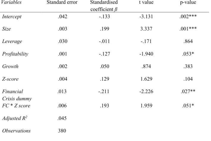
The sample for this study consists of 38 publicly listed Italian companies and the study period ranges from 2007 to 2017. Specifically, firms considered are classified as “mid cap” and the components of the FTSE Italia Mid Cap Index as of 31 December 2019 have been selected. The reason to consider exclusively mid cap companies is not fortuitous: the segment represents in our opinion the best scenario to investigate earning management and financial distress companies since it comprises many different kinds of firms - from those facing critical financial conditions, which have been excluded from the FTSE MIB Index, to those in excellent financial conditions that are experiencing a growth phase. Table 1 shows the industry-wide distribution of sample firms. As evident from the table, industrials and consumer industries are prevalent. We begin with an initial sample of 418 firm-year observations from 2007 to 2017 with available data to estimate the regression equations. Consistent with previous studies, we excluded from our sample companies operating in finance and banking industries because their financial statements respond to different rules and their accounting measures cannot be compared with those recorded by companies belonging to other industries. Certain other industries, such as
insurance and real estate and firms with missing or incomplete data have been excluded. We lost 38 firm-year observations because accruals variables in our equations needed to be deflated with lagged total assets data. We derived a final usable sample of 380 firm-year observations from 2008 to 2017. The data for the variables used in the study have been collected from the Osiris Database, a global corporate database provided by Bureau Van Dijk, and from Thomson Reuters Eikon for accounting data not available in the database.
Table 1. Industry-wide distribution of sample firms based on the industry classification benchmark (ICB)
Industry ICB Code No. of Firms
Oil & Gas 0001 4
Basic Materials 1000 1 Industrials 2000 15 Consumer Goods 3000 4 Consumer Services 5000 6 Telecommunications 6000 1 Utilities 7000 4 Technology 9000 3
Source: Author’s calculations.
3.2 Measurement of financial distress: Altman’s Z-score
Between the independent variables included in our models, the Altman’s Z-Score is the one of primary interest as it measures the firm’s level of financial distress. Even though the Z-score model was developed decades ago in 1968, it is the most widely used in the academic literature as a measure of financial distress and still accurate in assessing the overall financial health of the firm (Charitou & Lambertides, 2011), (Altman, 2017).
To predict whether the firm has a high probability of becoming insolvent or not, the score is based on five financial ratios: profitability, leverage, liquidity, solvency, and activity. Higher levels of the score denote a lower level of financial distress, whereas a lower score indicates a higher level of distress. Normally, an Altman Z-Score below 1.8 suggests a company might be headed for financial distress and eventual bankruptcy, while a score closer to 2.99 or higher implies the firm is financially strong.
It is estimated as follows:
Z - score = 1.2 (WC/TA) + 1.4 (RE/TA) + 3.3 (EBIT/TA) + 0.6 (MVE/TL) + 1.0 (Sales/TA) In this case:
WC = working capital, that is, current assets – current liabilities RE = retained earnings
EBIT = earnings before interest and tax MVE = market value of equity
TL = total liabilities TA = total assets
The first ratio, working capital over total assets, is a measure of the net liquid assets of the company relative to its total capitalisation. Working capital here is expressed as the difference between current assets and current liabilities. Generally, a firm facing operating losses will present shrinking current assets in relation to total assets. Comparing this liquidity ratio with current and quick ratios, this one proved to be the most valuable. Working capital over total assets explicitly considers liquidity and size characteristics.
Retained earnings over total assets is a measure of cumulative profitability over time. It is one of the two ratios introduced by Altman; the other is the use of market value of equity instead of the book value. The ratio implicitly considers the age of the firm due to its cumulative nature. A relatively young firm will show a lover RE/TA ratio as it takes time to increase its cumulative profits. Therefore, it may be stated that a young firm has a higher chance of being classified as bankrupt compared to another. But this is precisely how it works in real situations. The younger the firm, the higher the incidence of failure.
Earnings before interest and taxes over total assets ratio is a measure of the true productivity or profitability of the assets of the firm and it is not affected by any tax or leverage factors. Since the firm’s survival is dependent on the earning power of its assets, this ratio appears to be particularly suitable to determine insolvency.
Market value of equity (includes the combined market value of all shares, preferred and common) divided by the total liabilities shows the decrease in value of the assets before the liabilities exceed the assets and the firm goes bankrupt. The ratio adds a market value dimension to the model that other studies did not previously include. The debt to equity ratio, which is widely used nowadays to measure financial leverage, is the reciprocal of this ratio.
The sales over total assets ratio is the standard capital turnover ratio and expresses the ability of assets to generate revenues. It assesses management’s capability in dealing with the competitive conditions a firm face. Because of its unique relationship to other variables in the model, the ratio is one of the variables that most contribute to the overall discriminating ability of the model, even though there is a wide variation among industries regarding asset turnover.
3.3 Measurement of Earnings Management
As previously mentioned in the literature review section, different models have been developed for the estimation of discretionary accruals, such as those by (Healy, 1985) (DeAngelo, 1986), (Jones, 1991), (Dechow, 1996) and the modified Jones model. Both the Jones model and modified Jones model has been extensively considered in the academic literature as effective models in the estimation of discretionary accruals (DA), considered as a proper proxy to measure earnings management. According to Dechow, the modified version delivers more powerful results than the original model. For this reason and because it relaxes the assumptions about the value of sales, the present article decides to adopt the modified Jones model to first compute the discretionary accruals.
First, total accruals have been calculated with the following formula: Tacct = ∆CAt - ∆Casht - ∆CLt + ∆DCLt - DEPt
𝑇acct = Total accruals in year 𝑡,
∆𝐶𝐴t = Change in current assets in year 𝑡,
∆𝐶𝑎𝑠ht = Change in cash and cash equivalents in year 𝑡,
∆𝐶𝐿t = Change in current liabilities in year 𝑡,
∆𝐷𝐶𝐿t = Change in short term debt included in current liabilities in year t,
𝐷𝐸𝑃t = Depreciation and amortization expense in year 𝑡.
According to the literature total accruals can be derived in two ways: by following either a balance sheet-based approach or a cash flow statement-based approach. The former formulates the total accruals as described above, the latter computes total accruals as the difference between net income and cash from operating activities. Healey and Jones used the balance sheet-based approach in their studies and therefore to be consistent in our research we decided to adopt the same approach.
Secondly, total accruals computed in year t then serve in the estimation of the modified Jones model, which is defined below:
TAcct /At-1 = α1 (1/At-1) + α2 (∆REVt – ΔRECt)/At-1 + α3(PPEt/At-1) + εt
In this case:
TAcct is total accruals in year t
At-1 is total assets in year t – 1
ΔREVt is the change in revenues from year t − 1 to year t
ΔRECt is the change in net receivables from year t − 1 to year
PPEt is property, plant and equipment plus long term deferred expenses in year t.
εt is the error term in year t.
Total accruals include variations in working capital elements, such as receivables, inventory and payables, which are influenced by changes in revenues (∆REVt). In order to control changes
in non-discretionary accruals determined by altered external conditions, we decided to include property, plant and equipment, long-term deferred expenses, as well as changes in revenues in
the model. Sales are also present in the model because this component is often subject to management manipulation as a way to show a sounder financial performance. The property, plant and equipment variable (PPEt), is necessary to control for the portion of total accruals
related to non-discretionary depreciation expenses.
The usual approach used in the literature for the estimation of discretionary accruals through a regression model is to consider it as the unexplained portion of total accruals. Since total accruals can be expressed into a discretionary and a non-discretionary component, the error term in the previous equation represents the estimated discretionary accruals (DA) component. The reason why all variables of the model are scaled by the lagged value of total assets is to reduce heteroskedasticity, which arises in statistics when the standard errors of a variable are non-constant over a specific amount of time.
3.4 Regression Models and Research Variables
The relationship between earnings management and financial distress for Italian mid cap firms is investigated using multiple regression analysis. First, we derived the following regression equation after controlling for the known determinants of earnings management in order to test our first hypothesis:
DAi,t = ß0 + ß1 Z SCOREi,t + ß2 SIZEi,t + ß3 LEVERAGEi,t + ß4 PROF + ß5 GROWTH + εt (1)
In this case:
DA = DA calculated using the Modified Jones model
Z SCORE = Altman Z-score as dummy variable. Coded 1 if < 1.8, 0 otherwise SIZE = Firm size measured as the natural logarithm of total assets
LEVERAGE = The ratio of long-term debt to total assets
PROFITABILITY = The ratio of net income to total assets (Return on Assets), in % points GROWTH = The ratio of market value of equity over book values of assets
Together with the Altman Z-score dummy, the regressions present a series of different control variables which are also used in other studies to explain the relationship of our interest. Indeed, to ensure the effect of our independent variable on the discretionary accruals is not influenced by external factors, other variables must be kept constant.
These control variables are described as follows:
SIZE, which is computed as the natural logarithm of total assets. According to other studies (Habib A., 2013), (Chen Y., 2010) the firm size is likely to have an impact on earnings management and therefore needs to be treated as control variable. Bigger firms not only have access to better controlling systems and first-class quality auditing services, but are also more concerned regarding the loss of reputation that can follows in case earnings management is detected than their smaller counterparts. For these reasons, it is assumed that firms with higher levels of total assets will engage in earnings management practices less, and that this phenomenon is more pervasive in small firms. Conversely, some authors state that larger firms are more likely to manage earnings than small sized firms. This can be the consequence of dealing with more pressure from financial markets if bigger firms have to meet or beat analysts’ expectations (Barton J., 2002), higher bargaining power with auditors and consequent negotiation in waiving earnings management attempts (Nelson, et al., 2002), more room to manipulate given the wider array of accounting treatments available and finally the possibility to lower political costs.
LEVERAGE: computed as long-term debt over total assets, expresses the leverage ratio of firms in the sample. This variable is expected to be positively correlated with discretionary accruals. Previous studies showed that as the relative level of debt rises, a firm is more likely to have tighter accounting constraints and therefore frequent accounting manipulation is often associated with firms characterised by high leverage (Press & Weintrop, 1990), (DeFond & Jimbalvo, 1994). Other studies (Sweeney, 1994) found that managers of firms approaching default conditions respond with income-increasing accounting changes.
PROF: profitability of the firm measured by return on assets (net income/total assets). (Nasuhiyah & Al., 1994) found that firms with lower profit margins hold earnings above certain levels in order to avoid the risk of reducing the firm’s value resulting from earnings fluctuation. Firms with low profit margins may therefore resort to earnings management in order to avoid this potentiality. (Chen & Huang, 2010) also choose return on assets as a control variable to proxy firms’ profitability.
GROWTH, which is the ratio between market value of equity and book value of assets, has demonstrated to have an influence on discretionary accruals. (Skinner, 1993) argues that high-growth firms are more likely to engage in opportunistic reporting behaviour. (Robin & Wu, 2012) examined how firm growth has an effect on the pricing of discretionary accruals and their
empirical tests reveal that the pricing is not significantly different between high and low growth firms. However, they also found that in high growth firms, positive discretionary accruals are priced to a greater extent in comparison with low-growth counterparts, while negative discretionary accruals are priced to a smaller extent. It is argued that that management of high growth firms may use discretionary accruals as a possible mechanism for signalling future performance of the firms.
To test if firms are more likely to engage in earnings management practices because they were previously involved in financial distressed condition, the following regression has been tested: DAi,t = ß0 + ß1 Z SCOREi,t-1 + ß2 SIZEi,t + ß3 LEVERAGEi,t + ß4 PROF + ß5 GROWTH + εt (2)
Dependent variable is discretionary accruals (DAt). The first model considers the Altman’s
Z-score (Z-Z-score) as a measure of financial distress at time t, while the second model uses the same explanatory variable but at time t-1 to see if firms, once they were in a financial distress condition in the previous year, go on to manage their earnings in year t. This type of analysis can be extremely useful for both regulators and stakeholders. In fact, if a positive correlation is found, it can be postulated that a delayed manipulation of earnings could conceal the negative effects of a distressed condition.
Finally, to test the incremental effect of the 2008 financial crisis on the relationship earnings management and financial distress, we added two variables to our first regression model:
DAi,t = ß0 + ß1 Z SCOREi,t + ß2 FCi,t + ß3 [FC*Z SCORE]i,t + ß4 SIZEi,t + ß5 LEVERAGEi,t +
ß6 PROF + ß7 GROWTH + εt (3)
4. Empirical results
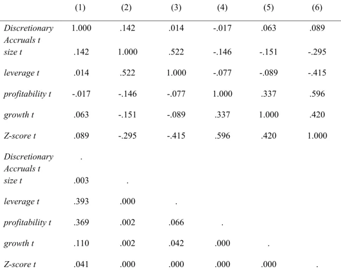
Before moving forward with the results of our OLS regressions, it is important to analyse the correlation matrix in order to check eventual multicollinearity between the variables of our regression equations. As the correlation table shows, none of the explanatory variables of our regressions presents correlation coefficients close to one in absolute value. According to the literature, only coefficients higher than 0.8 indicate significant multicollinearity between variables. Further, a variance inflation factor (VIF) has been calculated for all our models and it always showed a value close to two. We can therefore assume that multicollinearity between the independent variables is not an issue in our sample.
Table 2
Panel A: Descriptive Statistics
Variables Mean Median Std. Deviation Min Max
Discretionary Accruals .0176430 0.013815 .06529455 -0.44341 0.29367 Size 14.4344 14.395 1.30562 11.75 17.51 Leverage .1943 0.165 .14064 0 0.61 Profitability 4.4442 4.87 6.70199 -50.49 28.17 Growth 1.7761 1.335 1.61723 -1.08 14.15 Z-score .5421 1.72 .49888 -0.48 9.9
Panel B: Correlation analysis
(1) (2) (3) (4) (5) (6) DA (1) 1.000 Size (2) .142*** 1.000 Leverage (3) .014 .522*** 1.000 Profitability (4) -.017 -.146*** -.077 1.000 Growth (5) .063 -.151*** -.089* .337*** 1.000 Z-score (6) .089* -.295*** -.415*** .596*** .420*** 1.000
Panel A of the previous table contains the descriptive statistics of the independent variables used in our regression analysis while panel B reports the correlation analysis between these variables. From the descriptive statistics panel, a positive mean in DA indicates that, on average, firms in financial distress engage in income-increasing practices. Negative minimum value of
DA (-0.443) implies that firms also employ income-decreasing earnings management. The profitability of the sample firms presents a large standard deviation and it is the variable with the widest range between the minimum and the maximum value. This denotes that the ROA varies extensively across the sample firms. Wide changes across sample firms can be seen in respect of growth as well.
To better understand the strength of the linear relationship, we tested the significance of the correlation coefficients for the model. DA is positively correlated with Size (correlation coefficient significant at 1 percent level), which implies that bigger firms are more inclined to income-increasing earnings management practices. Our test variable Z-score, having a correlation coefficient of 0.089, is slightly positive but still significantly correlated at 10 percent level with DA. Z-Score is then strongly negative correlated with Size and Leverage and positively correlated with profitability and growth. All these coefficients are significant at 1 percent level.
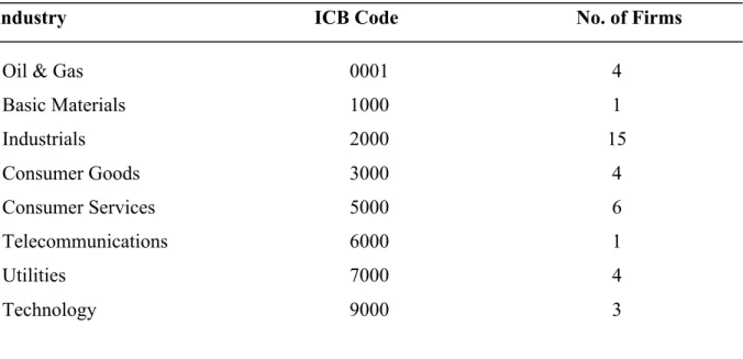
Table 3 reports the outputs for the relationship between discretionary accruals and financial distress throughout the timeframe considered. For our first regression in which Altman Z-score represents a proxy for the level of financial distress of the firms, our results reveal a positive and statistically significant relationship between the explanatory variable Z-score and the level of accruals of the firm. The coefficient is statistically significant at 1 percent level. The low adjusted R square (0.050) may indicate that the model does not fit well the data but these values are consistent with what calculated in previous studies if the Jones model has been applied in the computation of discretionary accruals (Siregar & Utama, 2008).
A positive standardized coefficient of the dummy variable Z-score implies that firms facing financial distress are more likely to adjust their earnings with the intention to improve the appearance of their financial statements. Therefore, we can confirm our first hypothesis, which assumes that firms in financial distress tend to be more involved in earnings management and accounting manipulation practices than firms with a stronger financial situation. This result suggests that companies in this distressed condition will presumably aim to conceal extreme levels of debt and poor results as a way to avoid further implications the firm may have with regulators and stakeholders. These results are consistent with what other authors discovered (Bisogno, 2015).
The second variable in the table, SIZE, also presents a level of significance at 1% and a positive coefficient, as expected. The implication here is that larger firms tend to employ higher levels
of earnings management, which should be reasonable, as these enterprises have more discretionary room. This fact appears to be consistent with what (Habib A., 2013) found in his research but inconsistent with the result of another paper (Bhattacharya, 2001), which found that smaller firms may show more frequent earnings manipulation practices because of higher levels of information asymmetry and lower requirements in terms of financial disclosure. The third variable, LEVERAGE showing a slightly negative coefficient, is not statistically significant. This result is in a certain way surprising because we should expect that high leverage firms are more likely to manipulate earnings over time in order to avoid debt covenant violations (Sweeney, 1994). Therefore, according to our model, we can assert that the level of a firm’s leverage does not have a significant impact on the level of earnings manipulation and cannot be considered as a good predictor of earnings management behaviours.
Finally, the fourth variable we want to discuss is a firm’s PROFITABILITY, measured by means on Return on Assets. This factor, which is statistically significant at 10 % level, shows a negative relationship with discretionary accruals and implies that less profitable firms tend to engage in earnings management actions in a way that hides poor short-term results, achieves target earnings and consequently reaches bonus compensation for the management.
Table 3 – Association between discretionary accruals (DA) and financial distress
***, **, *, Statistical significance at 1%, 5% and 10% levels of significance. T-statistics in parentheses; modified Jones discretionary accruals (DA) model is used to estimate earnings manipulation.
DAi,t = ß0 + ß1 Z SCOREi,t + ß2 SIZEi,t + ß3 LEVERAGEi,t + ß4 PROFt + ß5 GROWTHt + εt
Variables Standard error Standardized
coefficient ß t value p-value Intercept .042 -.140 -3.318 .001*** Size .003 .195 3.271 .001*** Leverage .030 -.013 -.203 .839 Profitability .001 -.122 -1.871 .062* Growth .002 .052 .918 .359 Z-score .004 .192 2.598 .010***
R2 .050
Observations 380
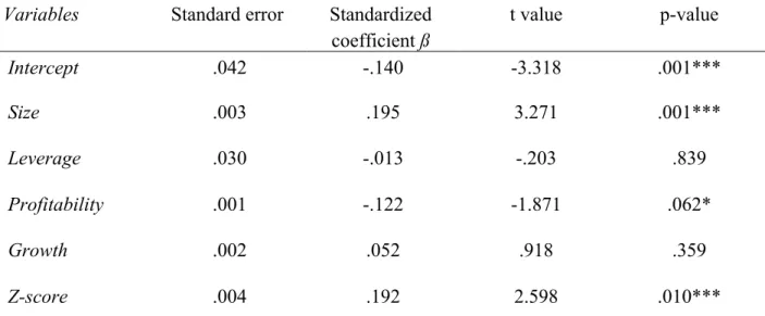
In the regression model 2, we want to analyse the relationship between financial distress and earnings management with a different timeframe. Z-score variable of the previous year is used. Here, our results are not statistically significant in terms of Z-score and thus we cannot consider this variable as a good predictor of earnings management practices. However, further studies with a higher number of observations are needed to test and verify this relationship. For variable SIZE the coefficient is found to be statistically significant at 1 per cent level, which is consistent with our previous and overall results.
Table 4 – Association between DA and financial distress one year behind
***, **, *, Statistical significance at 1%, 5% and 10% levels of significance. T-statistics in parentheses; modified Jones discretionary accruals (DA) model is used to estimate earnings manipulation.
DAi,t = ß0 + ß1 Z SCOREi,t-1 + ß2 SIZEi,t + ß3 LEVERAGEi,t + ß4 PROFt + ß5 GROWTHt + εt
Variables Standard error Standardized
coefficient ß t value p-value Intercept .043 -.127 -2.993 .003*** Size .003 .196 3.246 .001*** Leverage .030 -.062 -.966 .335 Profitability .001 -.049 -.814 .416 Growth .002 .085 1.543 .124 Z-score .003 .055 .826 .410 Adjusted R2 .035 Observations 380
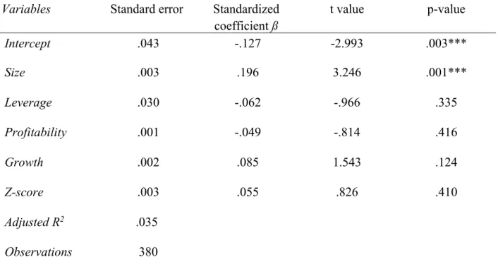
In table 5 we examine the relationship between earnings management and financial distress including in the regression a financial crisis dummy variable containing firm-year observations from 2008 to 2012, years in which the financial crisis affected the most Italian companies. To
test the incremental effect of global financial crisis on distressed firms’ discretionary accruals, this FC dummy has been combined with the Z-score. Results reveal that the Z-score, taken alone, does not show a significant relationship with our dependent variable but if we take into account the coefficients of the financial crisis dummy and the incremental effect FC * Z-score we reach statistically significant results. FC dummy, per se, is statistically significant at 5 percent level, while the combined variable is significant at 10 percent. The combined coefficient on (Z-score + FC * Z-score) is 0.451, a value 2.5 times higher than the ß coefficient of Z-score. This result highlights two facts: 1) a positive sign in the coefficient shows that firms in financial distress tend to manipulate their earnings more than non-financial distressed counterparts, which corroborated our first hypothesis; 2) distressed firms engage in income-increasing earnings management activities much more in periods of financial crisis.
Income-increasing earnings management is often seen in the literature as a potential red flag in the evaluation of financial reports because these are often measures used by listed firms to present the appearance of consistent income, smooth quarterly earnings fluctuations, and show to the market and to stakeholders a stronger financial position.
Between the other control variables of the model, SIZE and PROFITABILITY are the ones with statistically significant results. The bigger the size, the higher the level of DA, while the lower a firm’s return on assets, the greater the likelihood of manipulated figures.
Table 5 – Impact of the global financial crisis on the association between discretionary accruals and financial distress
Notes: ***, **, *, Statistical significance at 1%, 5% and 10% levels of significance. T-statistics in parentheses; modified Jones discretionary accruals (DA) model is used to estimate earnings manipulation.
DAi,t = ß0 + ß1 Z SCOREi,t + ß2 FCi,t + ß3 [FC*Z SCORE]i,t + ß4 SIZEi,t + ß5 LEVERAGEi,t +
ß6 PROF + ß7 GROWTH + εt (3)
Variables Standard error Standardised
coefficient ß t value p-value Intercept .042 -.133 -3.131 .002*** Size .003 .199 3.337 .001*** Leverage .030 -.011 -.171 .864 Profitability .001 -.127 -1.940 .053* Growth .002 .050 .874 .383 Z-score .004 .129 1.629 .104 Financial Crisis dummy .013 -.211 -2.226 .027** FC * Z score .006 .193 1.959 .051* Adjusted R2 .045 Observations 380
5. Conclusions
This paper provides evidence regarding the relationship between earnings management choices and financial distress condition in listed Italian firms with medium market capitalisation during the decade after the 2008 crisis. The study also considers whether this relationship changed during the global financial crisis. Based on the statistical results of our models we find that firms in financial distress, which are usually characterised by high leverage ratios, are more likely to disclose misleading account statements than financially ‘healthy’ firms. There are several reasons behind these actions: first and foremost, the ‘necessity’ to please analyst and shareholders’ forecasts and consequently to not affect the share price. Secondly, management remuneration is often tied to the firm’s accounting performance and therefore it is in managers’ interest to exaggerate accounting performance. This is often referred as the management compensation hypothesis (or ‘bonus plan’). Lastly, managers may report higher earnings in order to show better a liquidity position and avoid debt covenants violations (debt hypothesis). Among the control variables, Size has a significant positive relationship with earnings manipulation, implying that bigger firms have more incentives to manage earnings through DA. Profitability has a significant but negative relationship with DA. Finally, our last model shows that the level of accounting manipulation in the years of financial crisis is higher for distressed firms compared to firms in better financial conditions.
We believe the outcomes of our study have important implications not only for current and prospect investors but also for policy makers and regulators, who are responsible for monitoring financial reporting quality. Distorted accounting figures certainly mislead investors and make it harder to carry out a correct valuation of the future performance. Although our findings delivered interesting results, this study has some limitations. Firstly, a larger sample would probably provide more accurate results and a smaller margin of error. Secondly, due to unavailable data for the sample our models do not include cash flow as a control variable, but according to the earnings management literature this factor is a significant indicator of financial distress. Thirdly, expanding the analysis to a broader geographical base would probably deliver stronger results and this approach is therefore suggested for further research.
6. References
Altman, E. 2017. Distressed Firm and Bankruptcy Prediction in an International Context: A Review and Empirical Analysis of Altman’s Z-Score Model. Journal of International Financial Management and Accounting, 28(2).
Amara, I. 2017. The Effect of Discretionary Accruals on Financial Statement Fraud: The Case of the French Companies. International Research Journal of Finance and Economics, Issue 161. Barnea, A., Ronen, J. & Sadan, S., 1976. Classificatory smoothing of income with extraordinary items. The Accounting Review, Issue 51, pp. 110-122.
Barton J., S. P., 2002. The balance sheet as an earnings management constraint. The Accounting Review, Volume 77, pp. 1-27.
Bartov, E., 1993. The timing of asset sales and earnings manipulation. The Accounting Review, 68(4), pp. 840-855.
Bhattacharya, N., 2001. Investors' Trade Size and Trading Responses around Earnings Announcements: An Empirical Investigation. The Accounting Review, 76(2).
Bisogno, M., 2015. Financial Distress and Earnings Manipulation: Evidence from Italian SMEs. Journal of Accounting and Finance, 4(1).
Charitou & Lambertides, 2011. Distress Risk, Growth and Earnings Quality. Abacus, 47(2). Chen, K. & Huang, S., 2010. An appraisal of financially distressed companies’ earnings management: Evidence from listed companies in China. Pacific Accounting Review, Volume 22, pp. 22-41.
Christie, A. A., 1990. Aggregation of test statistics: An evaluation of the evidence on contracting and size hypotheses. Joumal of Accounting and Economics, 12(1-3), pp. 15-36. Cohen & Zarowin, 2007. Earnings Management over the Business Cycle. New York University Stern School of Business.
DeAngelo, H., DeAngelo, L. & Skinner, D., 1994. Accounting choice in troubled companies. Journal of Accounting and Economics, Volume 17, pp. 145-176.
DeAngelo, L., 1986. Accounting numbers as market valuation substitutes: A study of management buyouts of public stockholders. The accounting review, Volume 61, pp. 400-420.
Dechow, P., 1994. Accounting earnings and cash flows as measures of firm performance: The role of accounting accruals. Journal of Accounting and Economics, 18(1), pp. 3-42.
Dechow, P., 1996. Causes and consequences of earnings manipulation: An analysis of firms subject to enforcement actions by the SEC. Contemporary Accounting Research, 13((1)), pp. 1-36.
DeFond, M. & Jimbalvo, J., 1994. Debt covenant violation and manipulation of accruals. Journal of Accounting and Economics, Volume 17, pp. 145-176.
Ettredge, M., 2010. How Do Restatements Begin? Evidence of Earnings Management Preceding Restated Financial Reports. Journal of Business Finance & Accounting, pp. 332-355. Gul, F. A. & et al., 2003. Discretionary Accounting Accruals, Managers’ Incentives, and Audit Fees.
Habib A., B. M., 2013. Financial distress, earnings management and market pricing of accruals during the global financial crisis. Managerial Finance, 39(2), pp. 155-180.
Healy, P., 1985. The effect of bonus schemes on accounting decisions. Journal of Accountings and Economics, Volume 7, pp. 85-107.
Holthausen, R. & et al., 1995. Annual bonus schemes and the manipulation of earnings. Journal of Accounting and Economics, 19(1), pp. 29-74.
Jones, J., 1991. Earnings management during import relief investigations. Journal of Accounting Research, Volume 29(2), pp. 193-228.
Kaplan, R. S., 1985. Evidence on the effect of bonus schemes on accounting procedure and accrual decisions. Journal of accounting and economics, Volume 7(1), pp. 109-113.
Koch, A., 2002. Social Sciences Research Network, GSIA, pp. 2000-10. Levitt, A., 1998. The numbers game. The CPA Journal, 68(12).
McNichols, M. & Wilson, G. P., 1988. Evidence of Earnings Management from the Provision for Bad Debts. Journal of Accounting Research, Volume 26, pp. 1-31.
Nasuhiyah, A. & Al., 1994. Factors affecting income smoothing among listed companies in Singapore. Accounting and Business Research, Volume 24, pp. 291-301.
Nelson, Elliot & Tarpley, 2002. Evidence from auditors about managers’ and auditors’ earnings-management decisions. Accounting Review, Volume 77, pp. 175-202.
Palepu, K., 2016. Business analysis and valuation. 4th edition ed. s.l.:Thomson Learning. Press & Weintrop, 1990. Accounting-based constraints in public and private debt agreement. Journal of Accounting and Economics, Volume 12, pp. 65-95.
Rezaee, Z., 2005. Causes, consequences, and deterrence of financial statement fraud. Critical Perspectives on Accounting, 16(3), pp. 277-298.
Robin, A. & Wu, Q., 2012. Firm growth and pricing of discretionary accruals. Working Paper, Rochester Institute of Technology and Rensselaer Polytechnic Institute, Troy, NY.
Rosner, R., 2003. Earnings manipulation in failing firms. Contemporary Accounting Research, Volume 20, pp. 361-408.
Schipper, K., 1989. Earnings management. Accounting horizons, Volume 3, pp. 91-102. Siregar, S. & Utama, S., 2008. Type of earnings management and the effect of ownership structure, firm size, and corporate-governance practices: Evidence from Indonesia. The International Journal of Accounting, Volume 43, pp. 1-27.
Skinner, D. J., 1993. The investment opportunity set and accounting procedure choice: preliminary evidence. Journal of Accounting and Economics, Volume 16, pp. 407-445.
Smith, M., Kestel, J. & Robinson, P., 2001. Economic recession, corporate distress and income increasing accounting policy choice. Accounting forum, Volume 25, pp. 334-352.
Strobl, 2008. Earnings manipulation and the cost of capital. working paper, University of North Carolina at Chapel Hill, Chapel Hill, NC.
Sweeney, A., 1994. Debt-covenant violations and managers’ accounting responses. Journal of Accounting and Economics, Volume 17, pp. 281-308.
Young, S., 1999. Systematic measurement error in the estimation of discretionary accruals: an evaluation of alternative modelling procedures. Journal of Business Finance & Accounting, Volume 26(7‐8), pp. 833- 862.
7. Appendix
Table 6 – ANOVA results - First regression model
DAi,t = ß0 + ß1 Z SCOREi,t + ß2 SIZEi,t + ß3 LEVERAGEi,t + ß4 PROFt + ß5 GROWTHt + εt
Model Sum of Squares df Mean Square F Sig.
Regression .081 5 .016 3.940 .002
Residual 1.535 374 .004
Total 1.616 379
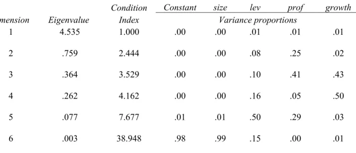
Table 7 - Collinearity diagnostics
Dimension Eigenvalue
Condition Index
Constant size lev prof growth
Variance proportions 1 4.535 1.000 .00 .00 .01 .01 .01 2 .759 2.444 .00 .00 .08 .25 .02 3 .364 3.529 .00 .00 .10 .41 .43 4 .262 4.162 .00 .00 .16 .05 .50 5 .077 7.677 .01 .01 .50 .29 .03 6 .003 38.948 .98 .99 .15 .00 .01
Table 8 - Correlations analysis (1) (2) (3) (4) (5) (6) Discretionary Accruals t 1.000 .142 .014 -.017 .063 .089 size t .142 1.000 .522 -.146 -.151 -.295 leverage t .014 .522 1.000 -.077 -.089 -.415 profitability t -.017 -.146 -.077 1.000 .337 .596 growth t .063 -.151 -.089 .337 1.000 .420 Z-score t .089 -.295 -.415 .596 .420 1.000 Discretionary Accruals t . size t .003 . leverage t .393 .000 . profitability t .369 .002 .066 . growth t .110 .002 .042 .000 . Z-score t .041 .000 .000 .000 .000 .
Table 9 - Anova results Second regression model
DAi,t = ß0 + ß1 Z SCOREi,t-1 + ß2 SIZEi,t + ß3 LEVERAGEi,t + ß4 PROFt + ß5 GROWTHt + εt
Model Sum of Squares df Mean Square F Sig.
Regression .056 5 .011 2.685 .021c
Residual 1.560 374 .004
Total 1.616 379
Table 10 - Model Summaryc
Model R R Square
Adjusted R
Square Std. Error of the Estimate .186b
.035 .022 .06458073
Table 11 - Collinearity diagnostics
Dimension Eigenvalue
Condition Index
Constant size lev prof growth
Variance proportions 1 4.535 1.000 .00 .00 .01 .01 .01 2 .759 2.444 .00 .00 .08 .25 .02 3 .364 3.529 .00 .00 .10 .41 .43 4 .262 4.162 .00 .00 .16 .05 .50 5 .077 7.677 .01 .01 .50 .29 .03 6 .003 38.948 .98 .99 .15 .00 .01
Table 12 - Residuals Statisticsa
Minimum Maximum Mean Std. Deviation N
Predicted Value -.0079449 .0562599 .0176430 .01215441 380
Residual -.44826847 .28956553 .00000000 .06415332 380
Std. Predicted Value -2.105 3.177 .000 1.000 380
Std. Residual -6.941 4.484 .000 .993 380
Table 13 - Descriptive statistics
DAi,t = ß0 + ß1 Z SCOREi,t + ß2 FCi,t + ß3 [FC*Z SCORE]i,t + ß4 SIZEi,t + ß5 LEVERAGEi,t + ß6
PROF + ß7 GROWTH + εt (3)
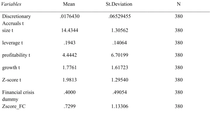
Variables Mean St.Deviation N
Discretionary Accruals t .0176430 .06529455 380 size t 14.4344 1.30562 380 leverage t .1943 .14064 380 profitability t 4.4442 6.70199 380 growth t 1.7761 1.61723 380 Z-score t 1.9813 1.29540 380 Financial crisis dummy .4000 .49054 380 Zscore_FC .7299 1.13306 380
Table 14 - ANOVA results Third regression model
DAi,t = ß0 + ß1 Z SCOREi,t + ß2 FCi,t + ß3 [FC*Z SCORE]i,t + ß4 SIZEi,t + ß5 LEVERAGEi,t +
ß6 PROF + ß7 GROWTH + εt (3)
Model Sum of Squares df
Mean
Square F Sig.
Regression .101 7 .014 3.549 .001c
Residual 1.515 372 .004
Total 1.616 379
Table 15 - Model Summary
Model R R Square Adjusted R Square Std. Error of the Estimate .250b