i
LAND CHANGE IMPACTS ON ECOSYSTEM SERVICES THROUGH
LANDSCAPE METRICS:
THE CASE OF MADEIRA ISLAND 1990-2040
ii
LAND CHANGE IMPACTS ON ECOSYSTEM SERVICES
THROUGH LANDSCAPE METRICS:
THE CASE OF MADEIRA ISLAND 1990-2040
Dissertation supervised by: PhD Pedro Cabral
NOVA Information Management School (NOVA IMS), Universidade Nova de Lisboa,
Lisbon, Portugal.
Dissertation Co - supervised by: PhD António Vieira
Department of Geography, University of Minho (UM), Guimarães, Portugal.
PhD Carlos Canut
Department of Mathematics, Universitat Jaume I (UJI), Castellon, Spain.
iii
ACKNOWLEDGMENTS
To the coordinators and staff of the Erasmus Mundus programme in Geospatial Technologies for the opportunity. To my supervisor Professor Pedro Cabral and co-supervisors Professor António Vieira, Professor Carlos Canut for their crucial insights, flexibility and support since the beginning of the project.
To Gabinete do Ensino Superior Madeira along with Câmara Municipal de Santa Cruz for the financial support.
To my classmates and friends specially Arman, Jonas, Laxmi, Mitzi, Nicodemus, Roberto, Stefana, William.
A special thanks..
To the ones that told me to go when the heart wanted to stay. Those who understood the purpose and the reason why. The ones that told me that I could. The ones that told me to believe. To the ones that told me to smile. To the ones that wanted this to happen although, not able to understand a single line.
The ones that told me to be myself. To the ones that told me to chase my dreams. To the ones that expected my presence when departing and arriving. To the ones that inspired me consciously or unconsciously. To the ones that told me that they were proud. To the ones that shared a piece of a journey since Santa Cruz, Funchal, Guimarães, Prague, Gaziantep, Lisbon and Münster…. still part of me.
To the ones that carried me in their arms and make me be, who I am…. Whom now, I carry in my mind and heart until we meet again:
Anabela Miranda Teixeira Nunes Maria Conceição Alves
iv
LAND CHANGE IMPACTS ON ECOSYSTEM SERVICES THROUGH
LANDSCAPE METRICS:
THE CASE OF MADEIRA ISLAND 1990-2040
ABSTRACT
LULC changes from anthropogenic disturbance are a major impact-driven on ecosystems services and landscape metrics have been proposed for the assessment of impacts depicting spatial patterns determining the quality and state of interactions.
Madeira island possesses a rich unique ecosystem the Laurel forest, a World Heritage inscribed by UNESCO. Along with a considerable amount of endemic biodiversity, fertile volcanic soils and humanized terraced landscape. Economic development and natural disasters have been triggering changes. Yet, future projections regarding LULC change are missing.
In this study, the CORINE Land Cover from 1990 to 2012 is used to perform change analysis. The Multilayer Perceptron Neural Network implement in the TerrSet GIS software is applied to model four scenarios for the year 2040: Business as Usual, Conservation of Agricultural and Forests areas and Renaturation with the assessment of impacts using landscape metrics. The results show a negative trend for ecosystem services in 2040 at different rates. A trend for the fragmentation of the landscape is found mainly in Renaturation scenario with 890 patches. A more significant decrease for biomass production in Scenario Renaturation and a loss of areas for food production of -32 km2 in Scenario Conservation of Forests. Recreational and cultural areas with a loss of -32 km2 in Scenario Business as Usual followed by Conservation of Forest with -29 km2.
This study contributes to Regional Planning Institutions improving monitoring and environmental resources management. Coupled with a practical application using landscape metrics for the assessment of ecosystem services accordingly with Burkhard and Maes (2017) in a context using future scenarios. Comparability from this study with other smalls islands can be performed.
v
KEYWORDS
CORINE Land Cover
Ecosystem services
Land use/ cover
Modelling
Landscape metrics
Scenarios
vi
ACRONYMS
CLC – CORINE Land Cover
GIS – Geographic Information Systems
LCM - Land Change Modeler
LULC – Land Use Land Cover
MPL – Multiplayer perceptron
vii
INDEX OF THE TEXT
1.Introduction ... 1 1.1Theoretical Framework ... 1 1.2 Objectives ... 6 1.3 Dissertation structure ... 6 2.Study area ... 7 2.1 Geographical context ... 7 2.2 Physical framework ... 8 2.3 Population framework ... 10
3.Data and methods ... 13
3.1 Data and tools ... 13
3.2 Methods ... 14
3.2.1 Modelling land use/cover change ... 15
3.2.2 Change analysis 1990 to 2012 ... 16
3.2.3 Change prediction and validation... 19
3.2.4 Impact of land change on ecosystems services ... 22
4. Results ... 24
4.1 Land change analysis 1990 to 2012 ... 24
4.2 Model validation ... 27
4. 3 Land change modelling 2040... 29
4.4 Impact of land change on ecosystems services ... 33
5. Discussion ... 36
5. 1 Land change analysis 1990 to 2012 ... 36
5.2 Land change modelling 2040 ... 37
5. 3 Impact of land change on ecosystems services ... 39
5.4 Limitations ... 45
5.5 Future recommendations ... 47
6. Conclusion ... 49
viii
INDEX OF TABLES
Table 1: Population and variation per municipalities Census 1991,2001 and 2011, in INE. ... 11
Table 2: Evolution of CORINE Land Cover (Buttner, 2014). ... 13
Table 3:Data and Sources. ... 14
Table 4: Shapefiles specifications used ... 14
Table 5: Driven variables. ... 18
Table 6: Elevation and slopes constraint. ... 20
Table 7: Validation measures.. ... 22
Table 9:Driven variable Cramer’s V results. ... 26
ix
INDEX OF FIGURES
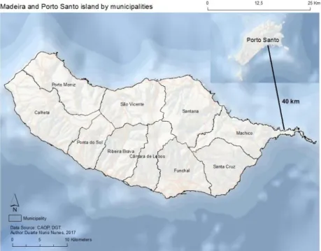
Figure 1: Geographic location of Madeira Island and municipalities. ... 7
Figure 2:Elevation per meters in Madeira Island. ... 9
Figure 3:Slopes percentages. ... 10
Figure 4:Population density in 2011 per km2 and municipalities. ... 11
Figure 5:Population variation rate 1991-2011, INE Census. ... 12
Figure 6: Land Change Modeler, workflow. ... 16
Figure 7: Land changes from 1990 to 2012, km2. ... 25
Figure 8: Change map 1990 to 2012. ... 26
Figure 9: Intensity analysis percentage of variation. ... 28
Figure 10: Error allocation and quantity. ... 29
Figure 11: Predicted changes Scenarios 2040, km2. ... 30
Figure 12:Transitions change map 2040 scenarios. ... 32
1
1. Introduction
1.1 Theoretical Framework
Land use and cover changes are accounted for the most important anthropogenic disturbance to the environment (Mishra and Rai, 2016) with profound impacts at the global scale (Foley et al., 2005). The ability and capacity for a progressive appropriation along with manipulation of space by man has been increasing in intensity and rate (Hassan et al., 2016; Geist, 2006). Driven factors in the demand for lands, such as proximity and socio-economic variables change the state result and spatial patterns (Geist,2005; Seppelt et al., 2016).
This led to a degradation of the environment, altering its functions, structures and dynamics (MEA, 2005; Grimm et al., 2008; Singh et al., 2014; Brandt et al., 2017; Grimm et al., 2008; Dong et al., 2015) disrupting the ecosystem function (Geist, 2006).
To maintain integrity of ecosystems is fundamental to preserve biodiversity (Singh et al., 2014; Brandt et al., 2017; MEA, 2005) and the services provided to society (Palacios-Agúndez et al., 2015) in terms of products obtained, benefits from the regulation, aesthetic experiences and recreation (MEA, 2005).
These concerns brought the environment to international agendas (Agenda 21, Paris Agreement), intergenerational awareness and Ecosystem Services Assessment (Millennium Ecosystem Assessment in 2005, Mapping and Assessment of Ecosystem and their Services in 2018).
The sustainable development goals in the 2030 Agenda by United Nations, empathizes the increasing awareness of including planning and monitoring of the landscape. With integrating ecosystems values and biodiversity in the national, regional and local planning (Addis Abeba Action Agenda, 2015).
Managing ecosystem services requires spatial knowledge of the dynamic patterns and their present status, its interactions (Leh et al., 2013). Plus, the LULC changes studies has been contributing towards the decision-making of ecological management and
2
environmental planning for the future (Zhao et al., 2004; Erle and Pontius 2007; Fan et al., 2007).
Remote sensing derived products along with geographical information systems, can perform integrated modelling building future scenarios with the applicability of probabilistic matrices which have been part of a wide range of studies assisting to explore the future of landscape (Rounsevell et al., 2006; Araya and Cabral, 2010) and measure of potential impacts (Shrestha et al., 2019).
Scenarios allow accounting an amplitude of plausible situation for the future, with the identification of losses and gains. It has been applied in several studies. For forest areas (Armenteras et al., 2019; Gibson et al., 2018) soil erosion (Jazouli et al., 2019) land degradation (García et al., 2019). To Luck (2012) most prioritization analysis for ESs is being based on the present state of LULC, a limitation for maintenance of ESs across time and implementation of strategies to mitigate impacts of land use change (Verhagen et al., 2018).
The importance of producing a predictive model of changes scenarios is the development of human activities and the consequent impact on environmental quality and the potential state of this landscape features in a later state (Sing et al., 2004). Several studies have been applied in future land cover transitions (Shrestha et al., 2019; Eraso et al., 2013; Weber et al., 2014; Guzmán et al., 2019; Kundu et al., 2017).
It allows to helping decision-making and the establishment protection and recovery actions (Muller and Burhard, 2012 in Almeida et al., 2016). An urgent need to identify the synergies existing between ecosystem services and ecosystem condition linking human activities effects creating priorities guidelines towards restoration (Mae et al., 2015). Studies showing the relation between the impact on land cover change on Ecosystem services (Metzger et al., 2006; Polce et al., 2016; Sturck et al., 2015).
Landscape metrics allows to describe the size, shape, the number of landscape elements (Turners, 1989, Turner and Garden, 1991) integrated into the landscape ecology studies for decades to quantify landscape structures (Casimiro, 2002). The fundamental characteristics are accordingly with McGarigal (1995) the structure related to the spatial
3
relationship of the elements or ecosystems in terms of dimensions, shape, number, type and configuration.
The analysis and interpretation range from the class levels and the whole landscape measuring the complexity, spatial distribution, diversity and composition (Leitão et al., 2006).
Although some uncertainties can rise for the selection and significance of individual indices (Schindler et al., 2014) it has been applied to assess impacts on ecosystem services for social mapping (Vreese et al., 2016) agricultural landscape (Lee et al., 2015) for evaluation of the landscape structures impact on biodiversity (Walz, 2015) estimation cultural scenic attraction (Walz and Stein, 2014). Current landscape patterns create legacies for the future (Turner and Garden, 2015).
Understanding the current state of the natural resources from which future goals can derive (Botequilha Leitão et al., 2006) from the thematic map or images (Herold et al., 2005). The spatial patterns compared to past trends and future predictions. These indicators allow to improve the aesthetic value of the landscape, assessment of ecological functioning (Frank et al. 2012) and quantify terrestrial and coastal ecosystem in a different temporal analysis (Cegielska et al., 2018; Uuemaa et al., 2009; Norris et al., 2010; Herold et al., 2005). Investigation of connectivity, fragmentation, configuration and complexity of ecosystem have been studied (Plexida et al., 2014; Tran and Fischer, 2017).
Burkhard and Maes (2017) state that landscape metrics are applied in several ecosystem services mapping and assessment for the environmental scientist, decisions makers. Despite its recognized potentiality studies using future scenarios are missing.
Its importance derives from the fact that allows helping decision-making process establishing protection and recovery actions (Muller and Burkhard, 2012 in Almeida et al., 2016). An urgent need to identify the synergies existing between ecosystem services and ecosystem condition linking human activities effects creating priorities guidelines towards restoration (Mae et al., 2015). Studies showing the relation between the impact on land cover change on Ecosystem services (Metzger et al., 2006; Polce et al., 2016; Sturck et al., 2015).
4
Islands also called biodiversity “hot spots” (Mittermeier et al., 1998 in MEA, 2005), due to their historical and evolutionary isolation, a unique endemicity in the species is found (Whittaker and Fernández-Palacios, 2007) with a finite space and movement capacity response to human-induced or natural disasters (Whittaker et al., 2001; Gillespie et al., 2008; Euroisles, 2002).
A continuous linkage between human pressure on terrestrial and marine ecosystems services occurs (MEA, 2005) resulting in increased vulnerability and species diversity pressure (Baldacchino, 2004). Despite this, they have been on the margin of the planning literature (Fernandes, 2017).
Many extinctions have already occurred on such islands occurring in a higher rate than in mainland’s system (MEA, 2005) because of land use changes and an introduction of predators and competitors (Sadler, 1989).
These changes have also occurred in the Macaronesia islands. This biogeographical region holds a significant level of biodiversity worldwide (Medail and Quezel, 1997; Borges et al., 2008; Santos et al., 2014) and important ecological structure (Cropper, 2013; Sundseth, 2009). Despite the minor dimension 0.2% in the global EU territory, owns the most endangered and vulnerable flora (Sundseth, 2009). Land-change studies are important to this region (Doulgas, 1997).
Several studies in islands context show the importance of information LULC historical changes analysis and land use patterns depicting environment state and human-induced effects on ecosystems (Mwalusepo et al., 2017; Kim 2016; Kim 2013; Leh et al., 2013) spatial pattern (Chi et al., 2019).
Madeira island, endemic flora, Laurel Forest, a 40-million-year-old primary forest ecosystem, the evergreen broadleaf trees, led the United Nation to inscribed as World Heritage in 1999 due to its “outstanding universal value”.
The IUCN World Heritage Outlook report in 2014 classified the trend of value of the forests has: “Good with some concerns” but in 2017 states: “High concern” because of deteriorating with the risk of fire, expansion of invasive species the increase of human usage (tourism and infrastructure development). In terms of overall threats, “a high
5
threat for prospects of land-use changes might further exacerbate these threats if protection and management do not account for these”.
A considerable amount of areas is part of the Natura 200 network, habitats directive and bird species directive (IFNC, 2019) along with a generous fertile soil for production of subtropical fruits and wine.
Tourism plays a major role in the regional economy, 25 to 30 % of its GDP (Neves, 2010) and its considered world’s leading island destination since 2015 (World Travel Awards, 2018). With a centenary tradition and one of the “oldest tourist destination” (Ismeri Europa, 2011). Nature-based tourism (ACIF, 2014; PENT, 2014) along with the unique landscape heritage of humanized agricultural areas and walks across nature, part of the island identity and cultural value (Vieira, 2017; Santos et al., 2014; Silva, 2013; Quintal, 2010). The laboured terrace agriculture landscape in the fifteen and sixteenth century, a tremendous endeavour engraved from a physical conditioned terrain (Kiesow and Bork, 2017).
A revolution of accessibilities through the application of sectorial European Union funds aiming Regional Development, occurs in the island in 1989, not to mention, the applicability in the development of new information and transportation technologies. With its first highway (VR1) after this, a succession of infrastructures (tunnels, bridges, roadways) will boost effect within the landscape in terms of transformation and dispersion of the human activities (Leitão, 2012). Likewise, an expansion of tourism, regional economy and transformation in the society (Dantas, 2012) coupled with demographical changes and internal migration movements.
Climate change projections were produced for the island (See Santos et al., 2014; Gouveia, 2014; CLIMA-Madeira, 2015) and land development pressure from 1990 to 2006 (Rodrigues, 2016). Yet, projections regarding LULC are missing in Madeira Island (Gouveia, 2014).
The present study intends to contribute for the lack of information regarding future LULC with spatial explicit scenarios of change and respective assessment with the application of the Burkhard and Maes (2017) methodology using landscape metrics for the ecosystem services impacts.
6
1.2 Objectives
The aim of this dissertation is to model four different spatial land use/land cover scenarios for the year 2040 in Madeira Island, with the identification of impacts on ecosystem services.
To achieve the proposed aim, the following specific objectives were defined:
• Analyze and identify change on LULC from 1990, 2000, 2006 and 2012 with CORINE Land Cover data, legend level 2;
• Develop from the 1990 and 2012 CLC four LULC scenarios for 2040: A business as usual; conservation of agricultural areas; conservation of forests areas and renaturation;
• Assess and identify major terrestrial ecosystem services impacts from 1990 to 2012 and scenarios with the use of landscape statistical metrics analysis.
1.3 Dissertation structure
The present dissertation is organized into six chapters. The first characterized by introductory theoretical framework, aim and objectives. The second presents the contextual geographical location of the study area, namely the physical framework and population framework. The third chapter, data and methods used in the developing of the practical component of the dissertation. The fourth chapter presents the several outcomes of this study and the fifth a discussion of the these. The last chapter presents the conclusions.
7
2. Study area
2.1 Geographical context
Madeira Island is a Portuguese Autonomous Region located in the Atlantic Ocean, distancing approximately 968 Km from Lisbon (southwest) and 800 Km northwestern from the African coast (Brandão, 1991) in the latitude 32° 42′ 0″ North and longitude 17° 0′ 0″ West. It is 504 km north of the Canary Islands and 980 km southeast of the Azores (Ribeiro, 1985).
Madeira region concerns the main island which is the most populated having a rectangle-like physical configuration reaching above the 1800 m with a length of 58 Km direction East to West. The total width corresponds to 23 km direction North-South (Ribeiro, 1949). Located 40 Km northeast is the island of Porto Santo and it includes the uninhabited natural protected island of Desertas and Selvagens (southeast). The total area corresponds to 740.2 km2 to Madeira and 42.5 km2 Porto Santo.
Madeira Island is divided into 11 administrative municipalities (Figure 1): Funchal the capital, Santa Cruz, Câmara de Lobos, Machico, Ribeira Brava, Calheta in the South part of the island. Santana, São Vicente, Porto Moniz and Ponta do Sol in the North part and Porto Santo.
8
2.2 Physical framework
Madeira island possesses a vigorous mountainous relief and consequently morphological declivity determinant in the whole landscape.
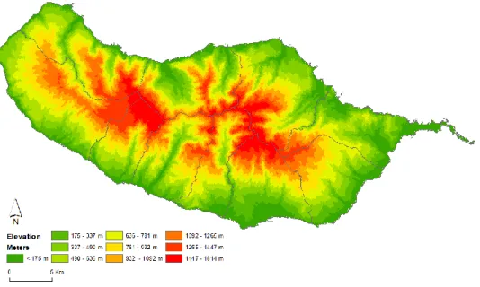
In terms of the elevation (Figure 2), higher points are in the central mountain range part appearing in a longitudinal backbone from East to West. Pico Ruivo with 1862 meters of altitude, Pico das Torres with 1851 meters and Pico do Areeiro with 1818 meters. There is a notorious division between the areas exposed to North and South in terms of its structure and climatic specificities. The north part of the island is characterized by the highest occurrence of sea cliffs drawn by polar winds, rain and a rough sea (Brito, 1997).
The south part is the opposite with less rain and a natural sheltered softer relief protected from the winds and possess higher temperatures. The climate condition of the island is influenced by its latitude and oceanic location, the proximity to African anticyclones and from Europe, the anticyclone of the Azores and the polar low atmospheric pressure at general scale (Quintal, 2007). The altitude and the exposure to solar radiation the global trade winds are the main local factors which influence the local climate.
The south part of the island is characterized by a higher number of hours exposed to the sun. The central backbone provokes the rapid rise of winds consequently, cloud formation and precipitation. The temperature is regular throughout the year decreasing with the altitude about 3°C by each 500 meters. The humidity and fog due to its orography constitute a high beneficial climatological factor in Madeiran vegetation (Pereira, 1989). Agricultural areas tend to be in the South part of the Island and East. Due to the climatic favourable conditions, in terms of higher temperature, fewer mists and fog (CLIMA-Madeira, 2015).
9
Figure 2:Elevation per meters in Madeira Island.
Approximately 7/10 of its surface area are higher than 25% of slope value being that 2/10 comprises between 25% and 16%. Only 1/10 of slope value equal or inferior to 16% (Brito, 1997).
The maximum value corresponds to 75%, its mean value 20% and the standard deviation is 12%. Natural factors print in the landscape irregular shapes due to physic and chemical interactions accelerating the erosive effects of wind, rain and sea (Ribeiro, 1999) in a continuous modelling of the topographical relief in terms of its structure and form (Abreu, 2008).
In Figure 3, visibly the South part of the island possess lower percentages of slopes as is the case of Funchal and Santa Cruz, although presents steep slopes in the form of valleys, which gives place in its end to streams with its origin in interior central areas. The central interior areas of the island are composed by high percentages of slopes due to its mountainous geomorphological structure.
The North part of the island possess a generally higher percentage of slopes comparatively with the South. The west-central part of the island is visibly composed by the largest plateau of Madeira with a total area of 24 Km2 and an average altitude of 1500 m.
10
Figure 3:Slopes percentages.
2.3 Population framework
When analysing the population census data for the years 1991 to 2011, produced by the national institute of statistics (INE) some important information related to regional demographical trend can be extracted (Table 1).
The total population for the year 1991 corresponded to 253 476 inhabitants, in 2001 a decrease for 245 011 and for the year 2011 an increase to 267 785 inhabitants. In terms of population is mainly, concentrated in the city of Funchal with 111 892 in 2011, followed by Santa Cruz that presents 43 005, Câmara de Lobos with 35 666, Ribeira Brava with 13 375, Calheta with 11 521 and Ponta do Sol with 8 862. In the North part of the island, Santana holds 7 719 inhabitants.
11 Municipality Population 1991 Population 2001 Population 2011 Variation rate 91-11 (%) Calheta 13 055 11 946 11 521 -12 % Câmara de Lobos Funchal Machico Ponta do Sol Porto Moniz Porto Santo Ribeira Brava Santa Cruz Santana São Vicente 31 476 115 403 22 016 8 756 3 432 4 706 13 170 23 465 10 302 7 695 34 614 103 961 21 747 8 125 2 927 4 474 12 494 29 721 8 804 6 198 35 666 111 892 21 828 8 862 2 711 5 482 13 375 43 005 7 719 5 723 13 % -3 % -1 % 1 % -21 % 17 % 2 % 83 % -25 % -25 % Total 253 476 245 011 267 785 6 %
Table 1: Population and variation per municipalities Census 1991,2001 and 2011, in INE.
The population density is higher in Funchal followed by Câmara de Lobos, Santa Cruz and Machico (Figure 4) with the rest of the island ranging 35 to 191 inhabitants per km2.
12
In terms of the population variation rate from 1991 to 2011 (Figure 5), a significantly higher percentage is found in Santa Cruz with 83% followed by the municipality of Câmara de Lobos with 13% and Ribeira Brava with 2%, meaning growth of population. On the contrary, the municipalities that lost a significant amount of population comprehends Santana with -25% and São Vicente with the same value. Followed by Porto Moniz with -21%. Calheta with -12%. Funchal with -3% and Machico with -1%.
13
3.Data and methods
3.1 Data and tools
During this study it was used data from several sources, the LULC from the CORINE Land Cover (Coordination of Information on the Environment) freely available (https://land.copernicus.eu/pan-european/corine-land-cover), providing information regarding LULC for many political directives (Water Framework Directive, Habitats Directive). Considered the most comprehensive dataset for terrestrial ecosystems at the EU level (Maes, 2018) and a major advance establishing a common methodology and classification in Europe (Geist, 2005).
It’s a product derived from remote sensing technology in which it has been maintained the same framework and resolution from 1990 until 2012 enable comparisons among Europe (Table 2). The minimum mapping unit is 100 meters.
Specification CLC 1990 CLC 2000 CLC 2006 CLC 2012
Satellite data Landsat 5 MSS/TM single date
Landsat 7 ETM single date
SPOT 4/5 and IRS LISS III dual date
IRS LISS III and RapidEye dual
date Time consistency 1986-1998 2000 +/- 1 year 2006 +/- 1 year 2011-2012
Geometric accuracy 50 m 25 m 25 m 25 m
Minimum Mapping Unit
100 m 100 m 100 m 100 m
Geometric accuracy 100 m Better than 100 m Better than 100 m Better than 100 m Thematic accuracy ≥ 85% (probably
not achieved)
≥ 85% (achieved) ≥ 85% ( not checked)
≥ 85%
Production time 10 years 4 years 3 years 2 years
Documentation Incomplete
metadata
Standard metadata
Standard metadata Standard metadata
Countries involved* 27 35 38 39
Table 2: Evolution of CORINE Land Cover (Buttner, 2014).
*Including late integration.
The Corine Land Cover is divided into three levels, the first level divided into 5 items with major categories the second level comprise 15 items and the third level with 44 items with a higher detailed categorization of the mapped features.
Table 3 presents the data and sources. Municipalities delimitation for a spatial explicit tool of analysis is used with the official government data of administrative limits. The digital elevation
14
model was used to derive elevation and slopes. Shapefiles from protected areas were provided by the official governmental institute of Madeira. The roads network was accessed with the Open Street Map information (https://www.geofabrik.de/data/download.html).
Data Format Source
Administrative Limits Shapefile General Directore of Territory
Corine Land Cover per year, 1990,2000, 2006,2012
Tiff Copernicous Monitoring Services Digital Elevation Model Tiff U.S. Geological Survey,
Aster Digital Elevation Model
Madeira Protected areas: Natura 2000, Natural Park, Natural reserves
Shapefile Institute of Forests and Nature Conservation, IP-Madeira
Roads network Shapefile Open Street Map
Table 3:Data and Sources.
The tools used during the execution of the present work was the GIS software ArcMap 10.5 and its Patch Analyst plugin by (Rempel, 2008) TerrSet with the Land Change Modeler (Eastman, 2016) and QuantumGIS 3.4.2.
3.2 Methods
The pre-processing part was done in the different Land Cover files, to extract the study area from the total raw extent included when using the CORINE Land Cover. The CORINE Land Cover of 1990, 2000, 2006, 2012, were reclassified from the legend level 3 to legend level 2. Where 12 classes are found in Madeira Island, and the class “burnt areas” was included in the “Open Spaces with little or no vegetation”, since only in the year 2012 this category appeared due to forests fires. All the shapefiles are integrated into the TerrSet software with the same parameters (Table 4), namely: legend; categories sequence; backgrounds value of zero; spatial dimensions in terms of resolution and coordinates
Settings
Columns: 558
Rows: 418
Resolution: 100 x and 100 y
No-data value: 0
Coordinate system: ETRS 1989 LAEA Extent:
Left: 1788904.1054 Top: 1544630.9392 Right: 1844704.1054 Bottom: 1592830.8392 Table 4: Shapefiles specifications used
15
The processing component was conducted in the Land Change Modeler an integrated LULC modelling and environmental assessment module (Eastman, 2016).
Exported to ArcMap 10.5 the application of the plugin Patch Analyst to calculate landscape metrics to assess impacts on ecosystem services. All the transitions below 1% of the total landscape was exclude from the analysis but presented in the annexes.
3.2.1 Modelling land use/cover change
The modelling was conducted in the Land Change Modeler of TerrSet. A stepwise process with the early map of CLC 1990 (time 1) and later map 2012 (time 2).
Fitted with the typical land change modelling process (Meyer and Turney 1992; Silva and Clarke 2002; Pontius and Chen, 2006), it was investigated quantitively land historical changes occurring in our study area and selected these transitions to build models for our scenarios. With this step, we produce a change map, as an input for the transitions sub-model. In transition sub-model, the transitions are grouped since empirically we assumed to be affected by the same driven factors for the changes (Eastman, 2016). Meaning that for example: a transition of heterogeneous agricultural areas to Urban fabric and/or forests to urban fabric are driven by the same variables.
Using the Cramer’s V measure, the assessment of driven variables is conducted to selected variables that possess a higher value of the measure which then explain the historical changes. The driven variables are then integrated into the change prediction, the Multilayer perceptron is used to produce a potential of land for a transition. With the potential of land for transition, it is possible to predict a future scenario for a specific date.
The model will determine how the driven variables influence future change, how much change took place between time 1 and time 2, and then calculate a relative amount of transition using Multi-Layer Perceptron Neural Network a powerful modelling tool (Bishop, 1995) to the future date with Markov chain matrix.
After this, a LULC for the year 2040 is produced and the interactive process with remodelling in transitions sub-model to simulate four different scenarios the main outputs (Figure 6).
16
Figure 6: Land Change Modeler, workflow.
The output was then exported to ArcMap 10.5 and the plugin Patch Analysist is used to calculated landscape metrics at the landscape level and class level.
3.2.2 Change analysis 1990 to 2012
The Land cover transitions from 1990 to 2012, were grouped into a single sub-model since the underlying driver of change is assumed to be the same for each transition (Pérez-Vega et al., 2012).
Diverse physical and human geography specificities of Madeira Island were considered to predict future changes for the period of 2040. Factors that potentially explain and consists in the main actors for the changes occurred among the period of 1990 to 2012, within the landscape.
Drivers of changes can be seen related to proximity factors or driving forces from which an impulse occur and change the state result (Geist, 2005) consisting in a GIS datasets representation (Pérez-Vega et al., 2012).
The selection of the driven variables was accounted from the general literature review (Olmedo et al., 2018; Mas et al., 2014) studies in Madeira Island (CLIMA-Madeira, 2015) and information from Regional governmental institutions (Institute of Forest and Nature Conservation), since specificities of the location and physical context rise the need to explore variables, which evokes the land change process, accounting assertive regional context.
17
The usefulness of each variable selected is identified with the use of Cramer V’s measures consisting in a product of a contingency table analysis (Eastman,2016) indicating the potential explanatory power of each selected variable. The variables consist of a separated shapefile. The measure ranges from 0.0 indicating no correlation to 1.0 corresponding to excellent explanatory power (Eastman, 2016; Megahed et al., 2015). In total it was created and tested 11 variables that were believed to drive the changes (Table 5).
Elevation of the island, since it ranges from 0 to 1862 meters, the assumption is that areas with a lower value of elevation are more susceptible to changes than higher values.
The slopes factor, since higher percentage of this variable, will be less suitable for changes. The distance to the coastal areas due to the development of economic and political activities near the coast, where historical settlements took a step for this tendency.
The distance to urban areas in 1990, we assume that areas that were closer to these areas were more vulnerable and likely to have transitions, a neighbouring effect of urbanization in which surrounding areas will suffer changes.
The distance to disturbance were agricultural areas and urban fabric from 1990 can drive the changes occurred until 2012, due to the proximity.
In the distance to roads variables, two main procedure was taken since the raw shapefile from Open Street Map, contained 23.936 polyline features for our study area. But, our intend analysis is to depict the effect of roads on driving the changes, consulting auxiliary documentation of Open Street Map, to guide volunteers, when attributing the classification per each polyline, accordingly with the description of no roads features, it was then removed the polylines classified has: path (1069 km); bridleway (658 m); track (468.8 km); track grade (169 km); steps (69 m); footway (375.6 km) ; pedestrian (40.30 km) and cycleway (1 km). Plus, the island possesses a significant number of tunnels, 452 with a total of 137 km. Not every tunnel is for traffic use, 160 features are integrated into paths a total of 29 km and
18
footways, with 37 features corresponding to 6.6 km. For traffic use, 249 features are integrated into highways with a total of 101 km. Being 2 of these tunnels with a length of 3 km, 7 with 2km and 16 with 1 km. It could not be assumed that the extension of the tunnel will affect changes, since they are underground passage way and enclosed, except the entrance and exit, then only the end and a start point of these features were considered. The distance to roads variables had a final value of 14.726 features.
Driven variable Assumption Source for
selection: Distance to capital Attractiveness factor Eastman (2016) Distance to coastal areas Change processes are increasing near
coast
CLIMA-Madeira (2005)
Distance to disturbance Agricultural and urban areas in 1990, closer areas will tend to be more vulnerable to change
Eastman (2016); Correia (2015) Distance to interior Change processes are increasing
towards interior areas, due to previous settlements near coast
CLIMA-Madeira (2015) and CMF (2014)
Distance to Natura 2000 Network
Proximity to protected areas Eastman (2016) Distance to Natural park Proximity to protected areas. Eastman (2016) Distance to roads Areas closer to roads will be more
likely affected by changes.
Eastman (2016); Leitão (2012); Cheng and Ding
(2016) Distance to South Location of 85% of the island
population
National Institute of Statistics Census 1991 and 2011. Distance to urban centres
in 1990
Areas closer to earlier urban centres have a higher change to be affected by urbanization
Eastman (2016)
Elevation Areas of low elevation will tend to suffer a higher rate of changes (e.g.: better climatic conditions)
Quintal (2007); CLIMA-Madeira (2015); Chen and Ding (2016) Slopes Areas with lower values will be more
likely to suffer change processes
Eastman (2016); Chen and Ding
(2016) Table 5: Driven variables.
19
3.2.3 Change prediction and validation
For the change prediction, it was applied the multilayer perceptron Neural network, a machine learning technique where the accuracy rate of the training should be achieved around 80% (Eastman, 2016). It consists of several interconnected nodes which are simple processing elements that respond to the weighted inputs received from other nodes (Atkinson and Tatnall, 1997). It uses several hidden layer nodes in which automatically evaluates and weights factor considering the correlations between the explanatory maps (Eastman, 2016). It flows unidirectionally from the input layer and the output layer (Du and Swamy, 2014; Bishop, 1995). Its performance depends not only of the choice of the driven variables, number of hidden layers, nodes and training data but also the training parameters such as the learning rate value, momentum controlling the weight change and the number defined of iterations (Mas et al., 2014; Taud and Mas, 2018). As suggested by Eastman (2016) the default values were used during this process.
In the MLP half of the training data are randomly selected for the learning process and other half for the validation. Testing how well the model performed at predicting change with the skill measure, consisting of the accuracy of transition prediction minus the accuracy expected by chance (Mas et al., 2014), ranging from -1 to +1 and 0 indicating a skill no better than random allocation (Eastman, 2016; Cohen, 1960).
It can handle multiple transitions at once and the explanatory variables are the same (Abuelaish, 2018). A multivariate function predicting the potential for a pixel to transition based of the values of the driven variables for that pixel (Eastman, 2016) the output consists in transitions potentials maps for each transition modelled with a continuous value from 0 to 1 (Eastman, 2016).
With the transition potential map, the Markov chain method is applied consisting in a probability of a system being in a certain state at certain time (Kamusoko et al., 2019) commonly used in land change models (Olmedo and Mas, 2018; Ozturk, 2015) and environmental modelling (Paegelow and Camacho, 2008).
The time set for the application of the probabilistic method is the year 2040, producing the probabilistic matrix of change determining the amount quantity of land for transition from one category to another in 2040 (Olmedo and Mas, 2018; Eastman, 2016) with a simple power of
20
the base matrix (Kemeny and Snell, 1976). It is produced two future land cover maps: soft prediction and hard prediction. The soft prediction is only the probability for a cell to experience land cover change. On contrary, the hard prediction identifies the new land cover based on multi-objective land allocation module (Eastman, 2016; Houet and Hubert-Moy, 2006).
The change prediction process integrated constraints (Table 6) the shapefiles specifically created, will consists in a mask: a value of 0 on areas treated as absolute constraints on the and value of 1 are unconstrained and able to suffer changes (Eastman, 2016) incorporated in the planning tab from the LCM. Given the regional context with a significant specific geomorphological structure, two main constraints variables were selected.
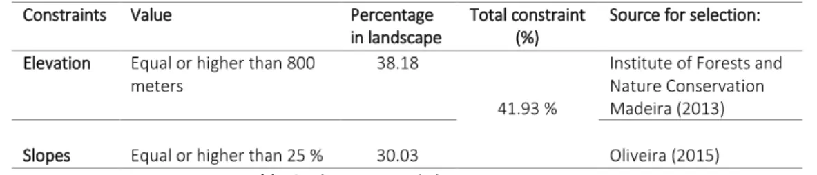
Elevation, since higher values of this variable, will not be suitable for land change, due to natural conditions with lower temperatures, a higher percentage of humidity but also anthropogenic factors, with low infrastructures and anthropogenic activities. At the same time, although the main human-induced changes have occurred within lower elevation areas, there is a need to consider the Laurel forest and transition areas of agriculture. The defined elevation range for no consideration of changes was 800 meters based on IFNC (2013). Another important factor to determine changes in the landscape is the variable of slopes. The assumption that lower values of slopes will be more likely to face changes.
The slope constraint selected was the value of 25%, based on Oliveira (2015) meaning that areas with this and higher value will not be considered to changes in our model and future scenarios.
The areas with these attributes will not be considered for future changes in our modelling process corresponding to 41.93% of our study area.
Constraints Value Percentage
in landscape
Total constraint (%)
Source for selection: Elevation Equal or higher than 800
meters
38.18
41.93 %
Institute of Forests and Nature Conservation Madeira (2013)
Slopes Equal or higher than 25 % 30.03 Oliveira (2015)
21
Four scenarios were modelled to 2040, with certain assumptions to explore plausible alternatives:
• Scenario Business as Usual (SC1): A continuation of the past changes; nature conservation is weak; little concern for biodiversity (Rounsevell et al.,2003); urban expansion; an increase of population.
• Scenario Conservation of Agriculture (SC2): Conservatives initiatives to protect these areas; Stimulation by European Union and Regional policies for production and integrity of agricultural activities.
• Scenario Conservation of Forests areas (SC3): Strict protection of areas with high biodiversity; Conservation policies and measures considered; Laurel forest protection. • Scenario Renaturation (SC4): Assertive population decrease prospects (DREM, 2018); stationary urban expansion; abandonment of agricultural areas; natural transitions (Shrubs to Forests; Shrubs to Open Spaces).
Using the CLC of 1990 and 2000 it was simulated a prediction for the year 2012 and compared with the actual real CLC 2012 for validation (Table 7). With this comparison, we calculate the number of correct predictions (Hits), the predicted persistence of areas (Null success) and errors due to observed change predicted to persist (Misses) and observed persistence predict as change (False alarms). Moreover, the identification and quantification of the error in terms of allocation and quantity allows to depict an overestimation or underestimation of the prediction. The intensity analysis in applied to identify if different intensity rates of change are influencing the prediction and its performance.
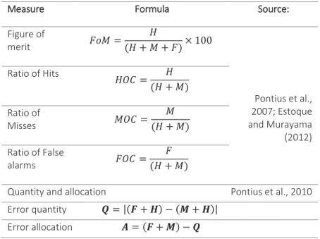
Three main approaches are performed to do validation: Figure of merit and ratios (Hits, Misses and False alarms) by Pontius et al. (2008) the intensity analysis by Aldwaik and Pontius (2012) and quantity and allocation proposed by Pontius and Millones (2011).
22
Measure Formula Source:
Figure of merit 𝐹𝑜𝑀 = 𝐻 (𝐻 + 𝑀 + 𝐹)× 100 Pontius et al., 2007; Estoque and Murayama (2012) Ratio of Hits 𝐻𝑂𝐶 = 𝐻 (𝐻 + 𝑀) Ratio of Misses 𝑀𝑂𝐶 = 𝑀 (𝐻 + 𝑀) Ratio of False alarms 𝐹𝑂𝐶 = 𝐹 (𝐻 + 𝑀)
Quantity and allocation Pontius et al., 2010 Error quantity 𝑸 = |(𝑭 + 𝑯) − (𝑴 + 𝑯)|
Error allocation 𝑨 = (𝑭 + 𝑴) − 𝑸 Table 7: Validation measures.
* H=Hits, M=Misses, F= False alarms
3.2.4 Impact of land change on ecosystems services
A considerable amount of metrics is available nowadays, as such the selection of variables that are appropriate to measure intending to achieve the desired ability to discriminate among different landscape types can be challenging. A further complication is to decide on an appropriate measurement scale. Spatial scale is known to affect observed patterns in landscapes (Wiens, 1989).
To assess the impact on ecosystem services it was used the landscape metrics referred in Burkhard and Maes (2017) in the CLC from 1990 to 2012 and from the predicted 2040 scenarios applied among the different classes accordingly with the author (Table 8). These metrics are applied in terms of the patch level and landscape level (McGarigal et al., 2002). The dimension of biodiversity using the Shannon’s Diversity Index in the landscape for all classes the patch density is represented with the number of patches since the landscape area is constant.
Provisioning services, with total patch area in km2 for potential production of biomass in forest areas class and production of food for the class arable land, consisting in the aggregation of the classes: Arable land; Permanent crops; Pastures and Heterogeneous Agricultural areas.
23
The assumption: increase of areas will allow a higher production and performance of the service.
Regulating service with Shannon’s Diversity index of agricultural areas to assess pest control and edge density of forests an effective tool for evaluating the effects of patch shape and area on the abundance of habitat edge (Hargis et al., 1998; Wallin et al., 1994) which is commonly used (Verhagen et al., 2018; Zulian et al., 2013; Bommarco, 2012).
Cultural services with a total of patch area of forest and arable land. Patch area for forest due to its touristic attractiveness factor and protected area (Van Berkel and Verburg, 2011) and agricultural areas represented by the same procedure has arable land. Limited information is available to assess cultural services in Europe (Maes et al., 2015). In our analysis we recognize the forest areas has a recreation opportunity (Maes et al., 2015), more land is protected and there is a positive trend in the opportunity for citizens and tourists to access these areas with significant recreation potential (Maes et al., 2015). Along with the laboured terrace agriculture landscape since in Madeira Island are part of the islander’s identity (Vieira, 2017; Kiesow and Bork, 2017; Santos et al., 2014; Silva, 2013; Quintal, 2010). Mean shape index of forest contributes to aesthetic value (Dramstad et al., 2006; Herbst et al., 2009) Further explanation of landscape metrics (see McGarigal, 2015).
Metric name Formula Units Description Use in ES (Burkhard
and Maes, 2017) Edge density (ED) 𝐸𝐷 = 𝐸 𝐴 (10,000)
E = total length (m) of edge in landscape
A = total landscape area (m2)
Meters per hectare
The total length of all edge segments per ha for the class or landscape of consideration (unit: m/ha). Regulating services: Habitat provision for pollination. Mean shape index (MSI) n MN = ∑ xij j=1 ni
Sum all patches ni = number patches same
type
Meters per hectare
Average complexity of patch shape for a class (the index is 1 when square, and increases without limit as the patch becomes more irregular). Cultural service: Landscape aesthetics Patch area (PA) 𝐴𝑖𝑗
Aij =area (m2) of patch ij.
Km2 Area (m2) of the patch. Provisioning
services: Production of food and biomass Patch density (PD) ni
Number of patches in the landscape of patch type (class) i
None Number of patches of the corresponding patch type.
Dimension of biodiversity: Landscape diversity
24 Shannon’s diversity index (SDI) m SHDI = ∑ (Pi * lnPi) i= 1 Pi = proportion of the
landscape occupied by patch type (class) i.
Information A measure of patch diversity in a landscape that is determined by both the number of different
patch types and the proportional distribution of area among patch types
Dimension of biodiversity: landscape diversity Regulating services: Pest control
Table 8: Metrics used for assessment of ecosystem services.
4. Results
4.1 Land change analysis 1990 to 2012
The most representative classes in Madeira’s landscape in 1990 was forests with 43% (316 km2), Shrubs/herbaceous vegetation with 25% corresponding to 188 km2, agricultural areas with 18% an area of 130 km2 and Urban fabric with 10% (72 km2) and the remaining 4% distributed by 8 classes, 35 km2.
The land change process in Madeira island is differentiated along the period analysed from the CORINE Land Cover, figure 7. From 1990 to 2000 the major change occurred in the urban fabric, with a total gain in percentage of the landscape being 3.92% representing 29 km2. The heterogeneous agricultural areas decreased its representativeness by -3.11% approximately 23 km2.
In the period 2000 to 2006, a percentage variation of 1.23% of Shrub class adding 9 km2 to the landscape. The urban fabric had a growth of 4.8 km2. Forest areas lost -4.41 km2 and agricultural areas, -2.88 km2.
From 2006 to 2012 a major loss of forest areas with -25.59 km2. Followed by Shrub class with -21.59 km2. The gains occurred mainly in the open spaces class with 46.83 km2. The changes in urban fabric and heterogeneous agricultural areas are residual.
25
Figure 7: Land changes from 1990 to 2012, km2.
The contributions for net change of the classes are: Heterogeneous agricultural areas to urban fabric with 26.9 km2; Forests to Urban Fabric with 3.22 km2; Forests to heterogeneous agricultural areas (3.34 km2); Forests to open spaces with 22.54 km2; Forests to Shrub with 4 km2; Pastures to Shrubs with 4.41 km2; Shrubs to Open spaces with 24.76 km2; Shrubs to Forest with 4 km2 and Heterogeneous agricultural areas to Shrub with 3.84 km2.
Spatially (Figure 8) the change map depicts a tendency in the south part of the island concentrated along Câmara de Lobos, Funchal, Santa Cruz, Machico and Santana, a higher prevalence of transitions from heterogeneous agricultural areas to the Urban fabric. Forests to Urban fabric located in Santa Cruz, Funchal, Calheta and Santana.
Forest to Heterogenous agricultural areas located mainly in the northwest of Calheta and Santa Cruz.
In the higher altitude areas of Funchal, Câmara de Lobos, Calheta the transitions from Forests to Shrubs, Forests to Open spaces, Shrub to Open spaces gains significance.
26
Figure 8: Change map 1990 to 2012
.
In the explanatory driven variables, elevation possesses the higher Cramer’s V measure meaning this natural variable is conditioning changes, followed by distance factors: to interior, urban centers in the year of 1990; to coastal areas; to south; to disturbance; to capital; to Natural 2000 Network; to roads, to natural park and finally slopes.
We can interpret that the changes and transitions that occurred in the period of 1990 to 2012 are being most influenced by these factors (Table 8).
Driven variable Cramer’s V
Elevation 0.2536
Distance to interior 0.2355
Distance to urban centers in 1990 0.2318 Distance to coastal areas 0.2088
Distance to south 0.2053
Distance to disturbance 0.1999
Distance to capital 0.1887
Distance to Natura 2000 Network 0.1778
Distance to roads 0.1628
Distance to Natural Park 0.1610
Slopes 0.1404
27
4.2 Model validation
The accuracy rate for our models (Table 9), had a higher percentage in SC2 with 83.95% followed by SC3 with 75.5% and finally SC1 with 71.67%. The decreasing value of the accuracy is related to the complexity of the transitions that were modelled, plus the ability of each variable to explain these transitions. This represents a positive accuracy rate, meaning that the variables selected to possess a strong explanatory power for the changes occurring in our study area.
Model Accuracy rate Skill measure/Kappa SC1 71.46 % 0.6789 SC2 83.95 % 0.7993 SC3 75.59 % 0.7071 SC4 71.67 % 0.6695
Table 9: Scenarios accuracy
Concerning the validation of our simulated LULC 2012 (Table 10)., a significantly low value of Figure of Merit is encountered 1.54% considered, a less than null model since the percentage is lower than 15% (Pontius et al., 2008).
.
Measure Result Figure of Merit 1.54 % Ratio of hits 0.02 Ratio of misses 0.98 Ratio of false alarms 0.29
Table 10: Validation measures results.
Since it was used the earlier CLC 1990 and CLC 2000, the remaining change a period from 2000 to 2012 is assumed to be the same.
As such the intensity analysis allow us to assess and depict the main trends on each period accordingly, with the intensity of land change (Pontius et al., 2013). Using the period rate (1990 to 2000) and comparing with 2000 to 2012, we can detect visually and quantitively, which pathway changes occurred more significantly (Figure 9).
28
Figure 9: Intensity analysis percentage of variation.
As such, we can see that different trends are taking place in terms of its intensity and per category.
First period (1990 to 2000) the main gain occurred in the Urban Fabric with 3.92% and the losses in Heterogeneous agricultural areas -3.11% and less significance for the forest (-0.61%) and residual value for Shrubs (-0.05%) and Open Spaces (0.06%).
In comparison with the period 2000 to 2012, an opposite trend occurred, an expressive higher gain in Open Spaces with 6.35% followed by Urban fabric with 0.68%. The losses occurred mainly in Forests (-4.97%) and Shrub (-1.69%). This shows that model accuracy is highly dependent on the comparison interval selected.
Applying the error allocation and quantity validation procedure we can identify an 83% of null success of correct observed and predicted persistence of the total landscape (Figure 10)., only 0.42% of correct observed change predicted as changes, 15.31% of error due to observed change predicted as persistence and 1.15% of error due to observed persistence predict as change. Our model predicted 1.67% of change and, occurred 15.73% of observed change from the CLC 2000 to CLC 2012. Our simulated 2012 underestimated the changes.
29
Figure 10: Error allocation and quantity.
Nonetheless, with intensity analysis and the good accuracy reached from the MLP and driven variables, it was decided to produce the scenarios for 2040 since it is intended to produce plausible scenarios for a distancing period of 28 years.
4. 3 Land change modelling 2040
In the urban fabric class, the SC1 present the higher value of variation with a growth of 33.62 km2, followed by SC3 with 29.74 km2, in lower value the SC2 with 0.49km2. This class is predicted to have a neutral change value for SC4. In terms of the results for the percentage of the total landscape in SC1, SC2, SC3 and SC4 it will represent 18.77%, 14.75%, 18.24% and 14.23%, respectively.
Heterogenous agricultural areas possess a decrease in every scenario except SC2, higher loss in SC3 with -37.24 km2, followed by SC1 with -23.37 km2 a value of -4.22 km2 for SC4, and a growth of 4.92 km2 in SC2. The percentage of the total landscape will correspond to 10.91 %, 14.72 %, 10.24 %, 13.49 % for SC1, SC2, SC3 and SC4.
30
Forests area predicted to decrease in the four scenarios being with higher intensity in SC4 with -5.62 km2, followed by SC2 with -3.23 km2 and SC1 with -1.24 km2. In the scenario SC3 the change is residual. The total landscape percentage for each scenario will be 36.72 % in SC1, 36.69 % in SC2, 37.87 % in SC3 and 35.86 % in SC4.
The class Shrub and Open spaces are predicted to possess changes a negative value of -25.09 km2 and a gain of 47.69 km2, respectively with Open spaces.
Figure 11: Predicted changes Scenarios 2040, km2.
When analysing spatially (Figure 12), we can depict a tendency for a continuous transition in the south part of the island.
Five main transitions are expected to occur in the Business as usual scenario (SC1): Heterogenous agricultural areas to Urban fabric with -23.37 km2, with significant transition in every municipality except Porto Moniz; Forest with a loss to Urban fabric and Heterogenous agricultural areas a total of -8.8 km2; Pastures to Shrub with -1.82 km2; Permanent crops to Urban fabric with -1.45 km2. Calheta municipality is exclusively presenting the transition from Forests to Urban fabric and Forests to Heterogeneous agricultural area with São Vicente. Concerning SC2, three main transitions are presented: Forests to Urban fabric with -3.88 km2 in Porto Moniz, Calheta, Santana, Machico and Ribeira Brava. Forests to Heterogeneous agricultural areas with -8.8 km2 in Calheta, Ponta do Sol, São Vicente. Pastures to Shrub with -1.82 km2 in the neighbouring of Calheta and Porto Moniz.
31
In SC3 three main transitions occur: Heterogeneous agricultural areas to Urban fabric with -28.29 km2 disperse across the island, higher areas of Santa Cruz, Câmara de Lobos, Ribeira Brava, Santana with lower expression in Machico and Funchal; Permanent crops to Urban fabric with -1.45 km2 located in the neighbouring limits of Funchal and Câmara de Lobos; Pastures to Shrub with -1.82 km2. On contrary to SC1, the north part of the island namely the municipalities of Porto Moniz and São Vicente presents the transitions from Heterogeneous agricultural areas to the Urban fabric.
For SC4, five transitions are predicted: Shrub to Forest and Open spaces with -34.58 km2 located mainly in the higher areas of Funchal, Câmara de Lobos, Santa Cruz and Santana; Forest to Open spaces with -20.99 km2 mainly in the south part of the island; Heterogenous agricultural areas to Shrub with -4.22 km2 distributed in São Vicente, Santana, Calheta, Ponta do Sol and Ribeira Brava.
32
33
4.4 Impact of land change on ecosystems services
Impacts of the land change on ecosystem services can be identified in Figure 13, representing the past and present trends with the 2040 scenarios comparison. The change is accounted for the reference year 2012.
The dimension of biodiversity, Shannon’s diversity measure in the landscape indicates a value of 1.47 in 1990, 2000 with 1.50, 2006 with 1.47 to 1.59 in 2012. Concerning the scenarios, the higher value is for SC4 with 1.64 followed by SC2 with 1.60 and SC1 with 1.58. The patch density is successively increasing from 381 in 1990 to 455 patches in 2012, with a significant increase for 2040 for all scenarios. A higher number is found in SC4 with 890 patches, followed by SC1 with 868, SC3 with 747 and finally the lower value, for SC2 with 660. In terms of the Forests patch numbers, it possesses 38 in 1990, 64 in 2012. For SC1 and SC2 a value of 123, 64 for SC3 and 153 for SC4.
For provisioning services, the patch area of arable land in the earlier year (1990) corresponded to 147 km2,it had a higher decrease in 1990 to 2000 corresponding to -26 km2, in which after had subtle variation until 2012, -11 km2. For 2040, a more significant decrease is excepted in SC3 (-32 km2) followed by SC1 (-27 km2) and SC4 with -6 km2, an increase of this area is expected in SC2 with 2 km2. Regarding forests patch area from 316 km2, a successive decreasing value is occurring from 1990 to 2012 a total of -36 km2, the period 2006 and 2012 indicates a clear negative fluctuation of -26 km2. A higher loss of this category is found in SC4 with -15 km2, a decrease similar values for SC1 and SC2 with -8 km2 and SC3 with a neutral value of 0.
Regulating services, Shannon’s diversity index of agricultural areas shows the increase from 1990 (0.47) to 2000 (0.48) and higher significant decrease change in the period 2000 to 2006 (0.24) and a value of 0.25 for 2012. Our scenarios predict a continuation of decrease mainly in SC1 with 0.15, following a smooth increase to 0.16 for SC3, in SC2 the value of 0.17 and SC4 with 0.18. The edge density of forests in 1990 is 17.92 meters per hectares, 18.4 in 2000, decrease to 17.03 in 2012. A higher value in SC1 with 17.95, SC2 with 17.6, SC3 with 17.03 and SC4 with 16.42 meters per hectares.
34
Cultural services, the patch area of the Agricultural and Forests had a total of 445 km2 in 1990. A higher decrease occurs in the first period to 2000 (-27 km2), -8 km2 to 2006, and -25 km2 until 2012. In the Scenarios a continuation of loss is predicted, more significantly in SC1 with -33 km2, followed by SC3 with -29 km2, SC4 with -19 km2 and -4 km2 for SC2. The mean shape index of forests decreased from 1990 (2.61) to 2012 (2.38). The same value is found in SC3, then a decrease for SC1 with 1.92, followed by SC2 with 1.93 and the lowest value in SC4 with 1.70.
35
Dimension of biodiversity
Provisioning services
Regulating service
Cultural service
36
5. Discussion
In this section it will be discussed the main outcomes from each step conducted in this study: historical land change analysis; land change modelling for the year 2040; assessment of the impacts on the different ecosystem services; limitations and recommendations for future work.
5. 1 Land change analysis 1990 to 2012
Identification of historical land changes in Madeira island from 1990 to 2012, assumes a clear opportunity to assess its implications while interpreting the dynamics driving the changes from human-induced and mix natural factors, a spatial informative source for intelligent regional planning application and intervention.
Our findings suggest that Madeira island had higher urban fabric growth, in the period of 1990 to 2000, with 3.92% of variation in the landscape in which after a stabilization occurred where, only 0.68% is found until 2012, probably explained by a low economic development and financial crises effects in Portugal (Carneiro et al., 2014; Rodrigues 2016).
This growth is spatially expressed in the south part of the island, mainly the neighbouring municipalities of Funchal. The establishment of new urban fabric towards higher elevation areas, in Santa Cruz and Câmara de Lobos, alike the population census variation rate, from 1991 to 2011, 83% and 13%, respectively (INE, 2011) and Leitão (2012). This tendency goes along with Azores islands (Gomes, 2013) and Europe trend from 2000 to 2010 (Maes et al., 2015) since the urban land had a growth of 0.35%. The urban fabric growth is occurring significantly from the heterogeneous agricultural areas (26.9 km2) followed by forest areas (3.22 km2) and permanent crops (2.97 km2).
The decreased of agricultural land coincides with European (Cegieslska et al., 2018; Gingrich et al., 2015; Levers et al., 2016) and global trends (Meiyappan et al., 2014). The most representative period is 1990 to 2000 where is presented -22.70 km2, after such the variation stabilize and turns to be residual (0.02%) due to the low expansion of urban areas. Nonetheless, new agricultural areas are emerging from forests areas (3.34 km2) in higher areas of Santa Cruz, and extreme northwest of Calheta municipality, effects of a decreasing available area.
37
The transition of Heterogenous agricultural areas to Shrub and/herbaceous vegetation representing -3.84 km2 is explained by the abandonment trend of these areas in the island (DREM,2011) along with Europe (Baumann et al., 2011) and Portugal mainland (Sturck et al., 2018; Eurostat, 2018). Furthermore, contrary to studies that show this abandonment trend contributing for growth of new Forest areas such as the island of Puerto Rico (Lugo and Helmer, 2004) and Quebec (Burton et al., 2003).
The forests areas which presented 42.64% of the total landscape in 1990, present a continuous significant decrease on contrary of Azores island (Gomes, 2013) and not meeting the European trend (except south) since studies indicate growth of these areas (Falcucci et al., 2007; Muchova and Tarnikova, 2018; Griffiths et al., 2013 in Cegieslaska et al., 2018; Mares et al., 2015) and even for future scenarios (Schroter et al., 2005). A variation of -4.68% for 1990 to 2012, but, significantly from 2006 and 2012 period, it presents a total loss of -3.46% (25.59 km2). Due to forest fires that significantly occurred on the island in 2012 (Liberato et al., 2017). The loss of these areas to Urban fabric, was 3.22 km2 with more spatial expression, in Santa Cruz.
A spatial dichotomy of the island manifests challenging fact to set planning instruments and protective actions of the natural heritage and convenient performance of conservation. If the coastal areas are being continuously under urbanization with more expression in the South part rising the influence under anthropogenic pressure, impacting terrestrial and pressuring coastal natural areas.
On the other hand, a trend of change towards the higher points (interior) of the island will lead to a loss of agricultural areas and forest areas. One of this, in the end, will suffer inevitable changes, the finitude of space determines. Our driven variables indicate that the distance to the interior is influencing more these changes.
5.2 Land change modelling 2040
Our first land change future model for Madeira Island depicts four scenarios in which planning mechanism and be conducted at the regional and local level. Since real policy decisions require two or more options to choose to account its future consequences (Corona, 2016) and our scenarios depicts differentiations in the intensity of changes notwithstanding, its locations.
38
Nevertheless, Scenarios needs to be “a coherent, internally consistent, and plausible description of a possible future state of the world”(Houghton 1995). All the scenarios are subjected and sensitive to the course of upcoming decades and has defined by Geist (2005) exogenous factors or forces (e.g.: economical; political).
The potential modelling is higher within 5 classes of the island since it possesses more area that transitioned, meaning that a higher number of cells can be considered when applying the MLP.
A scenario Business as Usual will result in predominate changes in the South part of the island, with upper areas of Santa Cruz, Câmara de Lobos, Ribeira Brava, Ponta do Sol having the change of Heterogeneous agricultural areas to the Urban Fabric. The transition of permanent crops to Urban fabric in the south-west of Funchal. Calheta with a significant coastal areas transition. An intensification of the historical changes is observed. This scenario implies an island population growth which is not prospected for 2040 (DREM,2017) but recent Madeiran emigrants return flows from Venezuela (6.000 people) in two years, and thousands of others across the world more than 420.000 (CCME, 2018), might drive new dynamics depending of the global geopolitical stability of the destination countries. The signs of economic growth (EC, 2017) and tourism will also be determinant.
A scenario of conservation of forests and agricultural areas will be dependent on pollical guidelines from European Union and sectorial funds for its application, and governmental aspirations from national, regional to the local level. And affects differently the landscape the growth is more spread in SC3 with the north part being part of transitions to the Urban fabric from Heterogeneous agricultural areas, differently from SC1.
The Scenario Renaturation intends to predict a continuous stationary urban growth, with major natural factors and abandonment of agricultural areas, playing a major role of changes since the same process that affects abandonment are the ones that drive conversion of land (proximity factors). Constraints were not accounted in the model and it depicts certain areas more likely to face abandonment of agricultural land (Santana, São Vicente, Ponta do Sol and Ribeira Brava) an explorative modelling that can serve to mitigate location more likely to suffer negative impacts.