Reciprocal recurrent selection effects on the genetic structure of tropical maize populations assessed at microsatellite loci

Reciprocal recurrent selection effects on the genetic structure

of tropical maize populations assessed at microsatellite loci

Luciana Rossini Pinto

, Maria Lucia Carneiro Vieira

, Claudio Lopes de Souza Jr.

and Anete Pereira de Souza

1

Universidade de São Paulo, Escola Superior de Agricultura “Luiz de Queiroz”,

Departamento de Genética, Piracicaba, SP, Brazil.

2

_{Universidade Estadual de Campinas, Centro de Biologia Molecular e Engenharia Genética,}

Departamento de Genética e Evolução, Campinas, SP, Brazil.

Abstract

A modified reciprocal recurrent selection (RRS) method, which employed one cycle of high-intensity selection, was applied to two tropical maize (Zea mays L.) populations, BR-105 and BR-106, originating the improved synthetics IG-3 and IG-4, respectively. In the present study the effects of this kind of selection on the genetic structure of these populations and their synthetics were investigated at 30 microsatellite (SSR) loci. A total of 125 alleles were revealed. A reduction in the number of alleles was observed after selection, as well as changes in allele frequencies. In nearly 13% (BR-105) and 7% (BR-106) of the loci evaluated, the changes in allele frequencies were not explained, exclusively due to the effects of genetic drift. The effective population sizes estimated for the synthetics using 30 SSR loci were similar to those theoretically expected after selection. The genetic differentiation (GST) between the synthetics increased to 77% compared with the original populations. The estimated RST values, a genetic differentiation measure proper for microsatellite data, were similar to those obtained for GST. Despite the high level of selection applied, the total gene diversity found in the synthetics allows them to be used in a new RRS cycle.

Key words: population genetics, plant breeding, molecular markers. Received: October 15, 2002; Accepted: June 26, 2003.

Introduction

Important increases in maize productivity have been obtained since the beginning of the last century because of the development of inbreeding and hybridization methods outlined by Shull (Crow, 1998). Currently, most maize breeding programs are based on hybrid production. The de-velopment of inbred lines and hybrids is very much related to the frequency of favorable alleles, which can be increased via recurrent selection (Hallauer and Miranda 1988). In this kind of selection, populations and inbred lines are developed to be crossed and to form superior hybrids. In the reciprocal recurrent selection method (RRS), genotypes from two ulations are evaluated in reciprocal crosses, where each pop-ulation is used as the other’s tester. The improved populations are generated by intermating superior genotypes of each population that present the best combining abilities with the reciprocal population (Souza Jr., 1998).

Similarly to selection methods, RRS causes changes in the allele frequencies, levels and distribution of the

ge-netic variability, and, consequently, in the gege-netic structure of the populations. The use of inadequate population sizes leads to the loss of genetic variability due to genetic drift ef-fects. Such loss can limit long-term RRS programs (Guzman and Lamkey, 1999, 2000). For this reason, high-intensity selection has been avoided in conventional RRS. However, Rezende and Souza Jr. (2000) applied one cycle of high-intensity RRS in the tropical maize populations BR-105 and BR-106 and, despite the negative drift effects on the improvement of the populationsper se, the inter-population genetic variances were not significantly af-fected.

Molecular markers are promising for the investiga-tion of all these changes. Labateet al. (1999) described sig-nificant changes in the allele frequencies at most maize loci after 12 cycles of RRS using the RFLP (restriction frag-ment length polymorphism) procedure, and genetic drift hypothesis was rejected by the Waples’ neutrality test (Waples, 1989a). Koeyeret al. (2001) identified genomic regions containing favorable alleles using 97 RFLP loci to monitor genetic changes in a long-term recurrent selection program in oats.

www.sbg.org.br

Send correspondence to Maria Lucia Carneiro Vieira. E-mail: mlcvieir@esalq.usp.br.

Currently, microsatellite markers are commonly em-ployed for the analysis of plant population genetic structure because of their co-dominant nature and high informative-ness. These markers represent non-coding DNA regions composed of small motifs of 1 to 6 nucleotides repeated in tandem, which are under mutation rates higher than those observed at the rest of genome (Jarne and Lagoda, 1996). Because of this, Slatkin (1995) proposed a genetic differen-tiation measure (RST) similar to Wright’s (1951) FST and Nei’s (1973) GST that seems more adequate for micro-satellite data analysis.

This study evaluated at the molecular level the effects of a high-intensity RRS cycle on the genetic structure of two important tropical maize populations, BR-105 and BR-106. Microsatellite loci were used to estimate (i) the change in allele frequencies after one cycle of selection, (ii) the genetic differentiation between the populations BR-105 and BR-106, and between their synthetics IG-3 and IG-4, expressed as GSTand RST, and (iii) the effective population sizes of the synthetics.

Material and Methods

Development of plant materials

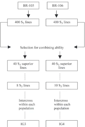
Two maize populations, a Thai (BR-105) and a Bra-zilian composite (BR-106) and their synthetics were ana-lysed. BR-105 and BR-106 were previously submitted to one cycle of high-intensity RRS (2.0 and 2.5%, respec-tively) using 400 S3lines. These lines were crossed with the opposite population and superior interpopulation half-sib (HS) progenies were identified. Eight S3lines (2.0%x400) derived from BR-105 and ten S3lines (2.5%x400) derived from BR-106, both related to the selected interpopulation HS progenies, were intercrossed in a diallel mating design within each population to develop IG-3 and IG-4 synthet-ics, respectively (Figure 1). The synthetics IG-3 and IG-4 resulted from intercrossing of S3linesi.e.they are the prod-uct of random mating of the alleles of eight lines derived from BR-105, and ten lines derived from BR-106, respec-tively. Considering that the effective population size (Ne) of each S3is approximately 0.57, theNeof IG-3 and IG-4 are 4.56 and 5.71 with inbreeding coefficients of 10.9% and 8.75%, respectively (Rezende and Souza Jr., 2000).

DNA extraction and SSR assays

One hundred randomly chosen seeds were taken from each population and synthetics. Leaf tissues collected from 35 day-old plants were lyophilized, ground by a mechanical mill, and stored at -20 °C. Total genomic DNA was ex-tracted from 300 mg of lyophilized tissues using a CTAB procedure (Hoisingtonet al., 1994). PCR reactions were performed in a 20µL final volume containing 40 ng of tem-plate DNA, 0.2µM of each forward and reverse primer, 100µM of each dNTP, 2.0 mM MgCl2, 0.5 unitTaqDNA polymerase (Gibco-BRL), 10 mM Tris-HCl and 50 mM

KCl. Reactions were run in a PTC-100 thermocycler (MJ Research) using the PCR cycling conditions described by Ogliariet al. (2000). Thirty primer pairs located at least in one maize chromosome were used to survey the genetic polymorphism. Amplification products were separated by electrophoresis on 3% agarose gels (50% agarose metaphor FMC-Bio products: 50% agarose Gibco-BRL) in TBE buffer (0,09 M Tris, 0,09 M boric acid, 2 mM EDTA). Gels were photographed under UV light after ethidium bromide staining. The sizes of the fragments were calculated by comparison with 50 and 100 bp ladders.

Statistical analysis

Allele frequencies

Individuals were genotyped in terms of their alleles and respective SSR loci, defined by a primer pair (for-ward/reverse). Allele frequencies were calculated using the BIOSYS-1 program (Swoffford and Selander, 1991). To test the hypothesis of identical distribution of the allele fre-quencies, an exact test for population differentiation was performed with the TFPGA program (Miller, 1997). The neutrality test (Waples, 1989a; Labateet al., 1999) was ap-plied to each locus to verify whether the changes in allele

frequencies after one cycle of RRS could be exclusively at-tributed to the genetic drift effects.

Diversity distribution

The distribution of gene diversity was conducted ac-cording to the model proposed by Nei (1973), in which the total genetic diversity mean (HT) is partitioned in two com-ponents: the gene diversity mean within population (HS), and between populations (DST). The proportion of total gene diversity (GST) between population, or genetic differ-entiation, was calculated as GST= DST/HT. To better under-stand the behavior of gene diversity after one cycle of selection, total gene diversity was performed separately for populations (before selection - C0), and for synthetics (after selection - C1), as well as for the combinations BR-105vs. IG-3, and BR-106 vs. IG-4 using the FSTAT program (Goudet, 1995). Genetic differentiation was also estimated by using the RSTstatistics, as the fraction of total variance in the allele size (in base pairs) that occurs between popula-tions, using the RSTCALC package (Goodman, 1997).

Effective population size

IG-3 and IG-4 effective population sizes (Ne) were estimated according to the Waples method (1989b), based on Plan II, where the individuals are taken before the repro-duction event, and not replaced. ConsideringN0andNtas

the respective sampling sizes at the two sampling events, t the time between the two sampling events, and Fc$ the weighted standardized variance in allele frequencies,Neis given by

$ $

Ne t

Fc

N Nt

= − −       2 1 2 1 2 0

The standardized variance in allele frequencies for each locus (Fc) was calculated using the expression pro-$ posed by Nei and Tajima (1981):

$ ( ) ( ) ( ) ’ ’ ’ Fc p p p p p p u u u k u u u u u k = − + − = =

∑

∑

wherepuandp’uare the frequencies of theuallele at the two

sampling events andkis the number of alleles at a locus. For multiple loci,Fc$ is given by the weighted means of sin-gle locus values (Fc) by the number of alleles at each locus.$ The 95% confidence intervals were calculated using the formula:

IC95 2 2

0 005 0 995

%, $ $ , . , , $ , . , Ne kNe k kNe k =      χ χ

based on the number ofkindependent alleles (

∑

(

)

Results

Allele frequencies

The 30 loci revealed a total of 125 alleles, 111 occur-ring in BR-105 and 116 in BR-106 (Table 1). Most of the alleles that were in low frequency in the original popula-tions were lost after one cycle of RRS. Allele reducpopula-tions were observed in IG-3 (23%) and IG-4 (17%). An increase in the number of alleles belonging to the extreme classes of frequencies was detected in both populations after selection (Figure 2). This is a feature of a dispersive process in which the allele frequencies tend towards the limits of zero (lost) or 1 (fixation). The differentiation tests for the allele

fre-Table 1- Allele frequency distribution (p$u) in two maize populations (BR-105 and BR-106) and their synthetics (IG-3 and IG-4) according to the microsatellite locus.

BR-105 IG-3 BR-106 IG-4

Loci (Bin) Alleles (bp) p$u

a

CI95% p$u CI95% p$u CI95% $pu CI95%

Bnlg 109 344 0.364

n = 92

(0.300; 0.438) 0.435

n = 92

(0.367; 0.510) 0.222

n = 90

(0.171; 0.290) 0.271

n = 94 (0.214; 0.341) (1.02) 388 0.505 (0.436; 0.580) 0.565 (0.496; 0.638) 0.661 (0.593; 0.727) 0.367 (0.303; 0.440) 438 0.011 (0.003; 0.039) 0.000 - 0.111 (0.075; 0.166) 0.261 (0.204; 0.329) 632 0.120 (0.081; 0.175) 0.000 - 0.006 (0.001; 0.029) 0.101 (0.003; 0.038)

Phi 001 76 0.353

b n = 95

(0.290; 0.425) 0.745

n = 92

(0.681; 0.806) 0.126

n = 87

(0.085; 0.182) 0.183

n = 93 (0.135; 0.246) (1.03) 86 0.374 (0.310; 0.447) 0.000 - 0.184 (0.136; 0.248) 0.075 (0.046; 0.123)

102 0.058 (0.033; 0.101) 0.027 (0.012; 0.062) 0.132 (0.080; 0.188) 0.000 -108 0.116 (0.078; 0.170) 0.228 (0.175; 0.296) 0.178 (0.131; 0.242) 0.220 (0.168; 0.287) 130 0.053 (0.029; 0.095) 0.000 - 0.092 (0.059; 0.144) 0.075 (0.046; 0.123) 154 0.047 (0.025; 0.088) 0.000 - 0.287 (0.224; 0.353) 0.446 (0.379; 0.521)

Bnlg 176 134 0.021

n = 94

(0.009; 0.054) 0.000

n = 96

- 0.010

n = 96

(0.003; 0.037) 0.005

n = 96 (0.001; 0.030) (1.03) 176 0.665 (0.598; 0.732) 0.995 (0.981; 0.999) 0.854 (0.802; 0.901) 0.984 (0.962; 0.997) 194 0.287 (0.229; 0.358) 0.005 (0.001; 0.029) 0.135 (0.095; 0.192) 0.010 (0.003; 0.039)

-Table 1 (cont)

BR-105 IG-3 BR-106 IG-4

Loci (Bin) Alleles (bp) p$u CI95% p$u CI95% p$u CI95% p$u CI95%

Bnlg 131 60 0.000

n = 94

- 0.000

n = 94

- 0.368

n = 95

(0.305; 0.441) 0.652

n = 96 (0.584; 0.718) (1.11). 84 0.064 (0.037; 0.108) 0.005 (0.001; 0.029) 0.137 (0.096; 0.194) 0.125 (0.086; 0.180)

96 0.362 (0.295; 0.430) 0.053 (0.030; 0.096) 0.084 (0.053; 0.133) 0.000 -102 0.117 (0.078; 0.170) 0.383 (0.318; 0.456) 0.195 (0.146; 0.258) 0.125 (0.086; 0.180)

116 0.074 (0.045; 0.120) 0.000 - 0.026 (0.012; 0.060) 0.000

-138 0.383 (0.314; 0.452) 0.559 (0.490; 0.631) 0.189 (0.141; 0.252) 0.099 (0.065; 0.150)

Bnlg 125 234 0.228

n = 90

(0.174; 0.296) 0.489

n = 92

(0.420; 0.564) 0.394

n = 94

(0.328; 0.467) 0.340

n = 94 (0.278; 0.413) (2.02) 258 0.061 (0.035; 0.107) 0.000 - 0.452 (0.385; 0.526) 0.218 (0.166; 0.284) 294 0.028 (0.012; 0.064) 0.000 - 0.048 (0.026; 0.090) 0.122 (0.083; 0.178) 324 0.400 (0.333; 0.475) 0.136 (0.094; 0.194) 0.032 (0.015; 0.068) 0.149 (0.105; 0.208) 348 0.283 (0.224; 0.335) 0.375 (0.310; 0.449) 0.074 (0.045; 0.122) 0.170 (0.127; 0.237)

Bnlg 108 78 0.032

n = 95

(0.015; 0.067) 0.000

n = 95

- 0.214

n = 90

(0.162; 0.277) 0.271

n = 94 (0.211; 0.340) (2.04) 100 0.826 (0.771; 0.877) 0.942 (0.905; 0.971) 0.464 (0.394; 0.534) 0.401 (0.334; 0.476) 106 0.142 (0.100; 0.200) 0.058 (0.033; 0.101) 0.313 (0.251; 0.381) 0.328 (0.267; 0.403)

116 0.000 - 0.000 - 0.010 (0.003; 0.037) 0.000

-MAGE05 98 0.526

n = 95

(0.458; 0.599) 0.163

n = 95

(0.118; 0.223) 0.758

n = 96

(0.696; 0.817) 0.813

n = 91 (0.755; 0.867) (2.05) 112 0.468 (0.401; 0.542) 0.837 (0.782; 0.886) 0.242 (0.188; 0.309) 0.187 (0.138; 0.251)

126 0.005 (0.001; 0.029) 0.000 - 0.000 - 0.000

-Bnlg 602 148 0.511

n = 93

(0.442; 0.585) 0.721

n = 86

(0.654; 0.786) 0.370

n = 96

(0.306; 0.442) 0.275

n = 89 (0.216; 0.347) (3.04) 154 0.269 (0.211; 0.339) 0.116 (0.077; 0.174) 0.307 (0.248; 0.378) 0.287 (0.226; 0.359) 168 0.134 (0.093; 0.192) 0.006 (0.001; 0.032) 0.198 (0.149; 0.261) 0.169 (0.121; 0.232) 172 0.086 (0.054; 0.136) 0.157 (0.111; 0.220) 0.125 (0.086; 0.180) 0.270 (0.211; 0.341)

Bnlg 197 84 0.199

n = 93

(0.149; 0.264) 0.022

n = 93

(0.009; 0.054) 0.016

n = 95

(0.006; 0.045) 0.011

n = 94 (0.003; 0.038)

(3.07) 98 0.000 - 0.000 - 0.179 (0.132; 0.241) 0.005 (0.001; 0.029)

108 0.000 - 0.000 - 0.089 (0.096; 0.194) 0.000

-120 0.462 (0.394; 0.537) 0.833 (0.778; 0.884) 0.674 (0.607; 0.740) 0.91 (0.865; 0.946) 126 0.339 (0.276; 0.411) 0.145 (0.102; 0.204) 0.026 (0.012; 0.060) 0.074 (0.045; 0.122)

132 0.000 - 0.000 - 0.016 (0.006; 0.045) 0.000

-n = 94 N = 96 n = 95 n = 95

MTTGBO2 150 0.232 (0.180; 0.301) 0.111 (0.073; 0.162) 0.128 (0.087; 0.182) 0.224 (0.174; 0.292)

(4.06) 165 0.111 (0.092; 0.190) 0.000 - 0.000 - 0.000

-174 0.247 (0.185; 0.307) 0.511 (0.443; 0.583) 0.144 (0.100; 0.200) 0.031 (0.015; 0.068)

195 0.089 (0.056; 0.141) 0.000 - 0.000 - 0.000

-228 0.321 (0.236; 0.396) 0.379 (0.311; 0.448) 0.729 (0.663; 0.788) 0.745 (0.691; 0.812)

Bnlg 589 154 0.372

n = 94

(0.308; 0.446) 0.833

n = 96

(0.779; 0.883) 0.226

n = 95

(0.174; 0.293) 0.672

n = 96 (0.606; 0.738)

(4.11) 162 0.000 - 0.000 - 0.321 (0.260; 0.392) 0.000

-170 0.537 (0.469; 0.610) 0.063 (0.036; 0.107) 0.179 (0.132; 0.241) 0.182 (0.135; 0.244)

210 0.000 - 0.000 - 0.274 (0.216; 0.343) 0.146 (0.103; 0.204)

232 0.090 (0.058; 0.141) 0.104 (0.069; 0.156) 0.000 - 0.000

-Bnlg 143 242 0.700

n = 95

(0.635; 0.764) 0.463

n = 94

(0.395; 0.537) 0.611

n = 95

(0.543; 0.680) 0.858

n = 81 (0.802; 0.908) (5.01) 256 0.300 (0.241; 0.371) 0.537 (0.468; 0.610) 0.084 (0.053; 0.133) 0.000

-280 0.000 - 0.000 - 0.305 (0.245; 0.376) 0.142 (0.097; 0.205)

Phi 113 96 0.284

n = 95

(0.226; 0.354) 0.125

n = 88

(0.085; 0.183) 0.263

n = 93

(0.207; 0.333) 0.000

n =

Table 1 (cont)

BR-105 IG-3 BR-106 IG-4

Loci (Bin) Alleles (bp) p$u CI95% p$u CI95% p$u CI95% p$u CI95%

Phi 48 188 0.033

n = 89

(0.016; 0.072) 0.000

n = 95

- 0.000

n = 95

- 0.000

n = 94 -(5.07) 196 0.815 (0.756; 0.869) 0.537 (0.468; 0.609) 0.347 (0.285; 0.420) 0.431 (0.362; 0.504)

220 0.152 (0.107; 0.213) 0.463 (0.396; 0.537) 0.653 (0.586; 0.720) 0.569 (0.501; 0.643)

Bnlg 238 134 0.353

n = 95

(0.290; 0.425) 0.042

n = 95

(0.022; 0.081) 0.005

n = 95

(0.001; 0.029) 0.000

n = 94 -(6.00) 150 0.084 (0.053; 0.133) 0.000 - 0.147 (0.105; 0.206) 0.101 (0.066; 0.153)

166 0.026 (0.012; 0.060) 0.163 (0.118; 0.223) 0.063 (0.037; 0.108) 0.053 (0.030; 0.096) 184 0.105 (0.070; 0.158) 0.111 (0.074; 0.164) 0.300 (0.240; 0.371) 0.309 (0.248; 0.380) 194 0.379 (0.315; 0.452) 0.653 (0.586; 0.720) 0.347 (0.285; 0.420) 0.138 (0.097; 0.196) 228 0.053 (0.029; 0.095) 0.032 (0.015; 0.067) 0.137 (0.096; 0.194) 0.399 (0.333; 0.473)

Bnlg 161 120 0.353

n = 95

(0.289; 0.425) 0.000

n = 94

- 0.000

n = 91

- 0.000

n = 93

-(6.01) 138 0.063 (0.037; 0.108) 0.048 (0.026; 0.089) 0.000 - 0.000

-150 0.058 (0.033; 0.101) 0.149 (0.106; 0.208) 0.159 (0.114; 0.221) 0.086 (0.054; 0.136) 168 0.111 (0.074; 0.164) 0.298 (0.238; 0.363) 0.214 (0.162; 0.281) 0.070 (0.042; 0.120) 176 0.379 (0.315; 0.452) 0.505 (0.437; 0.579) 0.258 (0.201; 0.328) 0.360 (0.296; 0.434) 202 0.037 (0.018; 0.074) 0.000 - 0.231 (0.177; 0.299) 0.091 (0.058; 0.142)

224 0.000 - 0.000 - 0.137 (0.095; 0.196) 0.392 (0.261; 0.395)

Phi 70 80 0.548

n = 93

(0.479; 0.621) 0.618

n = 93

(0.550; 0.688) 0.557

n = 96

(0.489; 0.630) 0.526

n = 95 (0.458; 0.599) (6.07) 90 0.452 (0.384; 0.526) 0.382 (0.317; 0.456) 0.443 (0.375; 0.516) 0.474 (0.406; 0.547)

Bnlg 657 84 0.000

n = 92

- 0.000

n = 94

- 0.094

n = 96

(0.061; 0.144) 0.375

n = 96 (0.311; 0.448) (7.02) 94 0.190 (0.141; 0.254) 0.298 (0.238; 0.369) 0.292 (0.233; 0.361) 0.151 (0.108; 0.210) 98 0.516 (0.447; 0.590) 0.202 (0.152; 0.267) 0.302 (0.243; 0.372) 0.120 (0.082; 0.174) 104 0.114 (0.076; 0.169) 0.202 (0.152; 0.267) 0.214 (0.162; 0.278) 0.182 (0.135; 0.244) 116 0.179 (0.131; 0.242) 0.298 (0.238; 0.369) 0.099 (0.065; 0.150) 0.172 (0.126; 0.233)

Bnlg 155 92 0.763

n = 95

(0.698; 0.821) 0.422

n = 96

(0.356; 0.495) 0.442

n = 95

(0.375; 0.516) 0.511

n = 95 (0.442; 0.584)

(7.04) 108 0.026 (0.012; 0.062) 0.000 - 0.289 (0.231; 0.360) 0.000

-120 0.032 (0.015; 0.007) 0.161 (0.171; 0.221) 0.084 (0.053; 0.133) 0.000 -142 0.079 (0.051; 0.131) 0.177 (0.130; 0.239) 0.032 (0.015; 0.067) 0.000 -168 0.095 (0.059; 0.144) 0.240 (0.186; 0.306) 0.142 (0.100; 0.200) 0.484 (0.416; 0.558) 188 0.005 (0.001; 0.030) 0.000 - 0.011 (0.003; 0.037) 0.005 (0.001; 0.029)

Bnlg 572 84 0.261

n = 90

(0.204; 0.332) 0.368

n = 95

(0.305; 0.441) 0.541

n = 93

(0.469; 0.617) 0.815

n = 96 (0.757; 0.868) (7.07) 90 0.328 (0.265; 0.401) 0.105 (0.070; 0.158) 0.035 (0.016; 0.074) 0.011 (0.003; 0.039) 102 0.411 (0.345; 0.487) 0.526 (0.458; 0.599) 0.424 (0.355; 0.502) 0.174 (0.127; 0.237)

Phi 115 90 0.505

n = 95

(0.437; 0.578) 0.462

n = 93

(0.394; 0.537) 0.435

n = 93

(0.368; 0.510) 0.578

n = 96 (0.510; 0.649) (8.03) 120 0.495 (0.427; 0.568) 0.538 (0.468; 0.611) 0.565 (0.495; 0.637) 0.422 (0.356; 0.495)

Bnlg 669 108 0.368

n = 95

(0.305; 0.441) 0.807

n = 96

(0.750; 0.861) 0.559

n = 94

(0.490; 0.631) 0.826

n = 92 (0.769; 0.878)

(8.03) 114 0.047 (0.025; 0.088) 0.000 - 0.043 (0.022; 0.082) 0.000

-128 0.405 (0.335; 0.473) 0.182 (0.135; 0.244) 0.011 (0.003; 0.038) 0.043 (0.022; 0.084)

144 0.095 (0.061; 0.146) 0.000 - 0.005 (0.001; 0.029) 0.000

-160 0.074 (0.045; 0.121) 0.000 - 0.261 (0.204; 0.329) 0.016 (0.006; 0.047)

180 0.000 - 0.000 - 0.021 (0.009; 0.054) 0.000

-200 0.011 (0.011; 0.003) 0.010 (0.003; 0.037) 0.101 (0.066; 0.153) 0.114 (0.076; 0.169)

n = 92 n = 93 n = 95 n = 95

Bnlg 666 84 0.288 (0.229; 0.359) 0.258 (0.202; 0.327) 0.632 (0.564; 0.700) 0.274 (0.214; 0.339) (8.05) 126 0.288 (0.229; 0.359) 0.199 (0.149; 0.264) 0.100 (0.065; 0.152) 0.205 (0.153; 0.267) 138 0.092 (0.059; 0.144) 0.124 (0.084; 0.180) 0.111 (0.074; 0.164) 0.095 (0.061; 0.144) 166 0.293 (0.234; 0.365) 0.419 (0.353; 0.494) 0.158 (0.114; 0.218) 0.426 (0.356; 0.495)

186 0.038 (0.019; 0.077) 0.000 - 0.000 - 0.000

-Bnlg 240 112 0.100

n = 95

(0.065; 0.152) 0.068

n = 95

(0.041; 0.114) 0.313

n = 96

(0.252; 0.383) 0.339

quency distribution between the groups (Table 2) were highly significant (p < 0.01). Hence, despite the consider-able number of alleles shared between the original popula-tions, these populations differed greatly in allelic frequency. These differences between the original popula-tions and their synthetics could be attributed to the reduced number of lines intercrossed to form the synthetics. The changes in allele frequencies observed after one cycle of RRS (C1) were mainly due to the effects of sampling or ge-netic drift, since the Waple neutrality test was rejected by four loci in BR-105 and two loci in BR-106 (Table 3). These loci represent 13% and 7% of the total number in the synthetics IG-3 and IG-4, respectively. Changes in allele frequencies observed for the Phi 65 locus in IG-3 were complementary to IG-4.

Diversity distribution

The partition of gene diversity before selection (C0) showed that most of the gene diversity (89%) was within the original populations (Table 4). Similarly, after selection (C1), 80.5% of the total gene diversity found in the synthet-ics was distributed within them. Contrasting the values of total gene diversity mean (HT) before (C0) and after (C1) se-lection, we observed that nearly 10% was lost, while the mean gene diversity (HS) decreased 18% between C0and C1. Comparison of GSTvalues between C0(GST= 11%) and

Table 1 (cont)

BR-105 IG-3 BR-106 IG-4

Loci (Bin) Alleles (bp) p$u CI95% p$u CI95% p$u CI95% p$u CI95%

140 0.516 (0.447; 0.589) 0.542 (0.474; 0.614) 0.375 (0.311; 0.448) 0.557 (0.489; 0.629) 158 0.053 (0.029; 0.095) 0.000 - 0.271 (0.214; 0.339) 0.073 (0.044; 0.119)

n = 96 n = 96 n = 96 n = 96

MCTO2BO8 95 0.548 (0.479; 0.620) 0.753 (0.688; 0.810) 0.635 (0.564; 0.700) 0.578 (0.510; 0.649) (9.01) 125 0.452 (0.385; 0.526) 0.247 (0.195; 0.317) 0.365 (0.365; 0.304) 0.422 (0.356; 0.495)

Phi 65 130 0.797

n = 91

(0.737; 0.853) 0.346

n = 94

(0.285; 0.420) 0.626

n = 91

(0.557; 0.697) 0.646

n = 96 (0.579; 0.713) (9.03) 150 0.203 (0.152; 0.269) 0.654 (0.591; 0.725) 0.374 (0.308; 0.448) 0.354 (0.292; 0.426)

Bnlg 127 240 0.425

n = 93

(0.358; 0.499) 0.707

n = 94

(0.642; 0.771) 0.434

n = 91

(0.366; 0.509) 0.433

n = 90 (0.365; 0.509) (9.04) 252 0.575 (0.506; 0.647) 0.293 (0.233; 0.363) 0.346 (0.282; 0.420) 0.567 (0.496; 0.640)

264 0.000 - 0.000 - 0.198 (0.147; 0.263) 0.000

-276 0.000 - 0.000 - 0.022 (0.009; 0.055) 0.000

-Bnlg 292 120 0.689

n = 95

(0.624; 0.754) 0.984

n = 96

(0.963; 0.997) 0.921

n = 95

(0.881; 0.956) 1.000

n = 96 -(9.06) 152 0.311 (0.250; 0.381) 0.016 (0.016; 0.045) 0.079 (0.048; 0.126) 0.000

-Phi 59 144 0.000

n = 96

- 0.000

n = 90

- 0.031

n = 96

(0.015; 0.067) 0.000

n = 90 -(10.02) 162 0.321 (0.257; 0.380) 0.395 (0.328; 0.470) 0.318 (0.257; 0.389) 0.211 (0.159; 0.278)

171 0.679 (0.600; 0.737) 0.605 (0.536; 0.677) 0.651 (0.584; 0.718) 0.789 (0.728; 0.846)

Phi 84 150 0.703

n = 91

(0.637; 0.769) 0.952

n = 94

(0.919; 0.978) 0.705

n = 95

(0.640; 0.770) 0.598

n = 92 (0.529; 0.669) (10.04) 171 0.258 (0.201; 0.328) 0.005 (0.001; 0.029) 0.284 (0.224; 0.353) 0.342 (0.279; 0.416) 198 0.038 (0.019; 0.078) 0.043 (0.022; 0.081) 0.011 (0.003; 0.037) 0.060 (0.034; 0.104) c

(T) (111) (86) (116) (96)

a

CI95%: confidence intervals, b

n: sample sizes,cT: total number of alleles.

C1(GST = 19.5%) revealed an increase of 77.3%. Conse-quently, the synthetics became more divergent. Such allele losses contributed for this differentiation.

The genetic differentiation (GST) for the combina-tions BR-105vs.IG-3, and BR-106vs.IG-4 was greater for

the first group (12.4%vs.6.8%) in which the selection in-tensity was higher (2.0%vs.2.5%). These GSTvalues were statistically significant. The RSTvalues were slightly supe-rior to the GST values. As pointed out by Gaiotto et al. (2001) the RSTstatistic can be used as evidence of genotyp-Table 2- Differences in the allele frequency distribution in the four combinations between maize materials.

Combination BR-105vs.BR-106 IG-3vs.IG-4 BR-105vs.IG-3 BR-106vs.IG-4

p-value 0.00 0.00 0.00 0.00

df 60 60 60 60

a_χ2 _{539.87** 515.24** 561.01** 489.74**}

a_χ2_{test for allele frequency homogeneity: **significant at p < 0.01, df: degree of freedom.}

Table 3- Neutrality test for changes in allele frequencies after one cycle of RRS in the BR-105 and BR-106 maize populations.

BR-105/IG-3 BR-106/IG-4

Locus Bin N0 N1 χ2 Df N0 N1 χ2 df

Bnlg 109 1.02 92 92 0.98 3 90 94 5.65 3

Phi001 1.03 95 92 45.72** 5 87 93 4.12 5

Bnlg 176 1.03 94 96 3.43 3 96 96 15.79** 4

Bnlg 131 1.11 94 94 25.73** 4 95 96 0.55 5

Bnlg 125 2.02 90 92 7.84 4 94 94 4.02 3

Bnlg 108 2.04 95 95 0.73 2 96 96 0.10 3

MAGE05 2.05 95 95 2.35 2 95 91 0.17 1

Bnlg 602 3.04 93 86 2.30 3 96 89 0.70 3

Bnlg 197 3.07 93 93 4.60 2 95 94 6.10 5

MTTGBO2 4.06 94 95 1.55 4 94 96 0.48 3

Bnlg 589 3.07 94 96 1.04 2 95 96 2.47 3

Bnlg 143 5.01 95 94 2.23 1 95 81 0.71 2

Phi 113 5.03 95 88 2.62 3 93 91 1.88 3

Phi 48 5.07 89 95 2.93 2 95 94 0.31 1

Bnlg 238 5.03 95 95 4.71 4 95 94 1.47 5

Bnlg 161 6.01 95 94 1.60 5 91 93 1.73 4

Phi 70 6.07 93 93 0.16 1 96 95 0.04 1

Bnlg 657 7.02 92 94 6.26 3 96 96 0.79 4

Bnlg 155 7.04 95 96 3.91 5 95 95 7.82 4

Bnlg 572 7.07 90 95 1.95 2 86 92 27.29** 2

Phi 115 8.03 95 93 0.06 1 93 96 0.85 1

Bnlg 669 8.03 95 96 2.42 5 94 92 8.57 6

Bnlg 666 8.05 92 93 0.93 4 95 95 5.55 3

Bnlg 240 8.06 95 95 0.11 3 96 96 2.09 3

MACTO2BO8 9.01 94 95 1.40 1 96 96 0.14 1

Phi 65 9.03 91 94 10.48** 1 91 96 0.02 1

Bnlg 127 9.04 93 94 2.74 1 91 90 4.62 3

Bnlg 292 9.06 95 95 3.35 1 95 96 0.88 1

Phi 59 10.02 95 95 0.21 1 96 90 0.55 2

Phi 84 10.04 91 94 26.66** 2 95 92 3.25 2

ing accuracy due to the fact that its estimation is based on the magnitude of the variances.

Effective population size

The values for the effective population sizes esti-mated for the synthetics IG-3 (3.87) and IG-4 (6.62) were similar to those theoretically expected,i.e.for the recombi-nation of 8 and ten S3lines, respectively (Table 5). In prac-tical terms, it shows that the samples (on average 93 individuals) represent approximately 3.87 and 6.62 plants of an ideal panmitic population and correspond to 4.16% and 7.11% of the total sampled individuals from IG-3 and IG-4, respectively. The estimated effective population sizes provided inbreeding coefficients [(F = 1/2Ne).100] of 12.91% for IG-3 and 7.55% for IG-4, which are similar to the expected values of 10.94% and 8.75%, respectively.

Discussion

The differences in the allele frequency distributions between the original populations supported the existence of genetic divergence reported by Naspolini Filho et al. (1981) because of the magnitude of the heterosis mani-fested in the interpopulation cross.

Changes in allele frequencies between populations and respective synthetics were observed by the lack of overlapping of the confidence intervals in nearly 50% of the alleles. At most of the loci, the nature of these changes was due to stochastic processesi.e., genetic drift and sam-pling errors. Nevertheless, changes at some loci were highly significant, and therefore were not due to effects of drift alone.

The apparent lack of neutrality in RRS programs was verified by Labateet al. (1999) at 17% of the RFLP loci

dis-persed in the maize genome. This result was interpreted as a selection by genetic hitchhiking. As microsatellite loci rep-resent repetitive and non-coding DNA regions, they appar-ently are not subject to strong selection pressures (Heathet al., 1993). However, they can be linked to selected loci, and therefore subjected to selection by genetic hitchhiking.

The loss of total gene diversity detected at micro-satellite loci (9.4%) was similar to the decrease of genetic variance (8.8%) obtained for yield (Table 6). A similar re-sult was observed in the BSSS and BSCB1 maize popula-tions in which the loss of genetic diversity assessed at RFLP markers was consistent with the decrease in additive and dominant genetic variance in the BSSS population after 12 RRS cycles (Holthaus and Lamkey, 1995; Labateet al., 1999). Both studies confirmed that diversity, or expected heterozygosity, is proportional to genetic variance (Lacy, 1987).

Despite the intensity of the applied selection, our re-sults showed that the total gene diversity loss was not so large after one cycle of RRS. According to Rezende and Souza Jr. (2000), high-intensity RRS selection in BR-105 and BR-106 caused a significant increase in heterosis

Table 4- Mean values of gene diversity between the original populations BR-105 and BR-106 and their synthetics IG-3 and IG-4 after one cycle of RRS.

HS(CI95%) HT(CI95%) DST GST(*CI95%) RST(*CI95%)

BR-105vs.BR-106 0.57 (0.49; 0.64)

0.64 (0.57; 0.71)

0.07 11%

(0.08; 0.14)

11.4% (0.10; 0.13)

IG-3vs.IG-4 0.46

(0.39; 0.54)

0.58 (0.50; 0.65)

0.11 19.5%

(0.14; 0.26)

19% (0.17; 0.22)

BR-105vs.IG-3 0.50 (0.43; 0.57)

0.57 (0.50; 0.64)

0.07 12.4%

(0.09; 0.16)

11% (0.09; 0.13)

BR-106vs.IG-4 0.53 (0.46; 0.60)

0.57 (0.50; 0.64)

0.04 6.8%

(0.05; 0.09)

6.6% (0.06; 0.08)

*Bootstrap with 10.000 replicates.

Table 5- Effective population size (Ne$) for the maize synthetics IG-3 and IG-4. derived from BR-105 and BR-106. respectively.

Synthetics (N0; N1) _Fc$ Ne$ CI95%

IG-3 (93.50; 93.80) 0.14 3.87 2.90; 5.42

IG-4 (93.90; 93.50) 0.09 6.62 5.01; 9.14

$

Fc: mean standardized variance in allele frequency weighted over loci. N0; N1: number of individuals at the two sampling events: populations and

synthetics. respectively. CI95%: 95% confidence interval.

Table 6- Yield and genetic variance (σG 2

) for the original (BR-105 and BR-106) and selected (IG-3 and IG-4) maize interpopulations1_.

BR-105 BR-106 IG-3 IG-4 BR-105 x BR-106 IG-3 x IG-4

Yield*(Mg ha-1) 6.52 8.00 7.48 7.19 7.90 9.22

σG 2

(g p-1) - - - - 97.47 88.86

1_{Data from Rezende and Souza Jr. (2000).}

(25.7% for grain yield) and improved the cross perfor-mance between the synthetics IG-3 and IG-4, but the interpopulation genetic variances did not present signifi-cant changes (Table 6). The maintenance of genetic vari-ability has been reported in several long and short-term recurrent selection programs (Bernardo, 1996; Guzman and Lamkey, 1999), and by Labate et al. (1999), using RFLP markers. In addition, the use of large effective popu-lation sizes has shown no advantage for maintaining ge-netic variability for short-term recurrent selection (Guzman and Lamkey, 2000). The increase in the genetic differentia-tion (GST) after selection (77.3%)i.e., in the genetic diver-gence between the synthetics is predictable in a RRS program. The maintenance of two separate genetic pools al-lows different alleles to be fixed in each population and guarantees the heterozygous condition for these loci in the interpopulation hybrids. This situation can maximize heterosis whose expression considers the genetic diver-gence between populations and the dominance effects at-tributed to the heterozygous loci (Lamkey and Edwards, 1999).

In our results, microsatellites proved to be very prom-ising for monitoring genetic variability and gave support for the use of the improved synthetics in a next cycle of se-lection. In agreement with previous studies, short-term re-current selection does not require large effective population sizes, once the genetic variability is maintained at adequate levels after a high-intensity RRS procedure. We can con-clude that the modified RRS process, here investigated, would successfully replace the traditional RRS procedure in maize.

Acknowledgments

This work was partially supported by FAPESP. L.R.P. was supported by fellowship from CNPq.

References

Bernardo R (1996) Testcross selection prior to further inbreeding in maize: mean performance and realized genetic variance. Crop Science 36:867-871.

Crow JF (1998) 90 years ago: The beginning of hybrid maize. Ge-netics 148:923-928.

Gaiotto FA, Grattapaglia D and Vencovsky R (2001) Micro-satellite markers for heart of palm Euterpe edulis and E. oleracea Mart. (Arecaceae) Molecular Ecology Notes 1:86-88.

Goodman SJ (1997) RSTCalc: a collection of computer programs

for calculating estimates of genetic differentiation from microsatellite data and determining their significance. Mo-lecular Ecology 6:881-885.

Goudet J (1995) FSTAT (v. 12): a computer program to calculate F-statistics. Journal of Heredity 86:485-486.

Guzman PS and Lamkey KR (1999) Predicted gains from recur-rent selection in the BS11 maize population. Maydica 44:93-99.

Guzman PS and Lamkey KR (2000) Effective population size and genetic variability in the BS11 Maize population. Crop Sci-ence 40:338-346.

Hallauer AR and Miranda JB (1988) Quantitative Genetics in Maize Breeding. 2nd ed. Iowa State University Press, Ames, 340 pp.

Heath DD, Iwama GK and Devlin RH (1993) PCR primed with VNTR core sequences yields species specific patterns and hypervariable probes. Nucleic Acids Research 21:5782-5785.

Holthaus JF and Lamkey KR (1995) Population means and ge-netic variances in selected and unselected Iowa Stiff Stalk synthetic maize populations. Crop Science 35:1581-1589. Hoisington D, Khairallah M and González-De-León D (1994)

Laboratory Protocols: CIMMYT Applied Molecular Genet-ics Laboratory. CYMMYT, Mexico, p 51.

Jarne P and Lagoda PJL (1996) Microsatellites, from molecules to population and back. Tree 11:424-429.

Koeyer DL, Phillips RL and Stuthman DD (2001) Allelic shifts and quantitative trait loci in a recurrent selection population of oat. Crop Science 41:1228-1234.

Labate JA, Lamkey KR, Lee M and Woodman WL (1997) Molec-ular genetic diversity after reciprocal recurrent selection in BSSS and BSCB1 maize populations. Crop Science 37:416-423.

Labate JA, Lamkey KR, Lee M and Woodman WL (1999) Tem-poral changes in allele frequencies in two reciprocally se-lected maize populations. Theoretical and Applied Genetics 99:1166-1178.

Lacy RC (1987) Loss of genetic diversity from managed popula-tions: Interacting effects of drift, mutation, immigration, se-lection, and population subdivision. Conservation Biology 1:143-158.

Lamkey KR and Edwards JW (1999) The quantitative genetics of heterosis. In: Coors JG, Pandey S, Ginkel MV, Hallauer AR, Hess DC, Lamkey KR, Melchinger AE, and Stuber CW (eds) Proceedings of the International Symposium on the Genetics and Exploitation of Heterosis in Crops. CIMMYT, Mexico City, Mexico, 1997, pp 31-48.

Miller MP (1997) Tools for population genetic analyses (TFPGA) 1.3: a windows program for the analysis of allozyme and molecular population genetic data. http://www.public. asu.edu.

Naspolini Filho V, Gama EEG, Vianna RT and Moro JR (1981) General and combining ability for yield in a diallel cross among 18 maize populations (Zea maysL.). Revista Bra-sileira de Genética 4:571-577.

Nei M (1973) Analysis of gene diversity in subdivided popula-tions. Proceedings of the National Academy of Sciences of the USA 70:3321-3323.

Nei M and Tajima F (1981) Genetic drift and estimation of effec-tive population size. Genetics 98:625-640.

Ogliari JB, Boscariol RL and Camargo LEA (2000) Optimization of PCR amplification of maize microsatellite loci. Genetics and Molecular Biology 23:395-398.

Rezende GDSP and Souza Jr. CL (2000) A reciprocal recurrent selection procedure outlined to integrate hybrid breeding programs in maize. Journal of Genetics and Breeding 54:57-66.

Souza Jr. CL (1998) Seleção recorrente e desenvolvimento de híbridos. Reunión Latino Americana de Investigadores en Maiz. Santa Fé de Bogotá, Colombia, 1998, pp 18-19.

Swoffford DL and Selander, RB (1991) Biosys-1: a FORTRAN program for the comprehensive analysis for electrophoretic data in population genetics and systematics. Journal of He-redity 38:1358-1370.

Waples RS (1989a) Temporal variation in allele frequencies: test-ing the right hypothesis. Evolution 43:1236-1251.

Waples RS (1989b) A generalized approach for estimating effec-tive population size from temporal changes in allele fre-quency. Genetics 121:379-391.

Wright S (1951) The genetical structure of populations. Annals of Eugenetics 15:313-354.