Management Science Letters 5 (2015) 1081–1090
Contents lists available at GrowingScience
Management Science Letters
homepage: www.GrowingScience.com/msl
A methodology for quantitatively managing the bug fixing process using Mahalanobis Taguchi system
Boby Johna* and R. S. Kadadevarmathb
aSQC & OR Unit, Indian Statistical Institute, 8th Mile, Mysore Road, Bangalore, Karnataka State, 560 059, India
bDepartment of Industrial Engineering & Management, Siddaganga Institute of Technology, Tumkur, Karnataka State, 572103, India
C H R O N I C L E A B S T R A C T
Article history: Received March 5, 2015 Received in revised format August 16 2015
Accepted October 13 2015 Available online October 15 2015
The controlling of bug fixing process during the system testing phase of software development life cycle is very important for fixing all the detected bugs within the scheduled time. The presence of open bugs often delays the release of the software or result in releasing the software with compromised functionalities. These can lead to customer dissatisfaction, cost overrun and eventually the loss of market share. In this paper, the authors propose a methodology to quantitatively manage the bug fixing process during system testing. The proposed methodology identifies the critical milestones in the system testing phase which differentiates the successful projects from the unsuccessful ones using Mahalanobis Taguchi system. Then a model is developed to predict whether a project is successful or not with the bug fix progress at critical milestones as control factors. Finally the model is used to control the bug fixing process. It is found that the performance of the proposed methodology using Mahalanobis Taguchi system is superior to the models developed using other multi-dimensional pattern recognition techniques. The proposed methodology also reduces the number of control points providing the managers with more options and flexibility to utilize the bug fixing resources across system testing phase. Moreover the methodology allows the mangers to carry out mid- course corrections to bring the bug fixing process back on track so that all the detected bugs can be fixed on time. The methodology is validated with eight new projects and the results are very encouraging.
Growing Science Ltd. All rights reserved. 5
© 201
Keywords: Bug fixing Software testing
Mahalanobis Taguchi system Design of Experiments K-Nearest Neighbour classifier
1. Introduction
Quality, cost, schedule and functionality are the critical factors for the success any software project (Tian, 2005). The quality of software is often expressed in terms of defect density,which is defined as the number of defects per unit size in the software (Fenton & Pfleeger, 1996). Since software development is a human activity, it is not possible to completely prevent the injection of defects (Jalote, 2000). Hence the best way to ensure the quality of software is to detect and fix the defects or bugs before releasing the software.
* Corresponding author.
E-mail address: [email protected]; [email protected] (B. John) © 2015 Growing Science Ltd. All rights reserved.
1082
The bugs are generally detected through reviews and testing during the software development life cycle. The software testing is the process of determining whether the software meets the needs of the customers and if it doesn’t, then reporting the bugs (Perry, 1995). The software testing involves the execution of test cases with the selected inputs, observing the actual outcome and verifying that the actual outcome is same as that of the expected outcome (Naik & Tripathy, 2008). The test cases (TCs) need to be designed in such way to capture as many bugs as possible. Moreover all the detected bugs need to be fixed before the release of the software to ensure the quality and prevention of software failures.
The system testing or the final phase testing of complete, integrated software plays a crucial role on software release. If large number of bugs is detected towards the end of system testing then the bug fixing may delay the software release or result in releasing the software on time with compromised functionalities. I.e. removing the software components with open bugs and releasing the software. Both the scenarios are undesirable and can lead to customer dissatisfaction, cost overrun and loss of market share. The proper scheduling of test case execution and optimum allocation of resources and efforts for bug fixing across system testing can prevent these problems. Unfortunately many Indian software companies fail to release the software on time due to the presence of open bugs (bugs detected but not fixed) at the scheduled time of software release. The software company for which this research project is undertaken has been able to release only 67% of the software on time with full functionalities due to the problem of open bugs. Hence there is a need for developing a methodology for quantitatively managing the bug fixing process across system testing phase so that the bugs can be fixed on or before the scheduled release of the software.
Many research works have been carried out in the past in the field of software quality and reliability engineering. The focus of these works is on developing prediction models for software defects or reliability. These models are needed to judge whether software is reliable or free from bugs. But to release the software on time with full functionalities, controlling of sub processes in software development life cycle, especially bug detection and bug fixing processes are necessary. Not many research works have been carried out on controlling or quantitatively managing the software life cycle phases. Most of these works (Weller & Card, 2008; Jacob & Pillai, 2003; Raczynski & Curtis, 2008; Humphrey, 1988; Harter et al., 2000; Jiang et al., 2004; Agarwal & Chari, 2007; Rao, et al., 2008; Boby & Kadadevaramath, 2013; Boby & Kadadevaramath, 2014) are on controlling the bug detection processes or establishing the relationship between process maturity, quality, cycle time, etc. Hence this research is undertaken to develop a methodology to quantitatively manage the bug fixing process during system testing to prevent the problem of open bugs at the time of software release.
The reminder of the paper is arranged as follows: details of data collected are given in session 2, session 3 describes the study methodology used for identifying the critical factors impacting the on time release of the software. The bug fixing process management methodology is described in session 4. The validation of the proposed methodology is given in session 5. The conclusions are given session 6.
2. Data collection
from that of unsuccessful ones. Hence the authors have decided to use a multidimensional pattern recognition approach, namely Mahalanobis-Taguchi system (MTS) methodology, to differentiate the successful projects from the unsuccessful ones. The details of MTS methodology and why MTS is chosen over other pattern recognition or classification techniques is given in the next session.
Table 1
Data on bug fixing progress at different % of TC execution
Project ID
% of TCs Executed
Project Status
10% 25% 50% 60% 70% 80% 90% 100%
1 0.00 0.63 0.60 0.69 0.57 0.79 1.00 0.97 Successful
2 0.07 0.71 0.58 0.72 0.63 0.81 0.94 0.99 Successful
3 0.10 0.65 0.56 0.61 0.63 0.88 0.92 1.00 Successful
4 0.00 0.63 0.45 0.69 0.74 0.86 0.94 0.97 Successful
5 0.10 0.64 0.62 0.63 0.65 0.88 0.93 0.99 Successful
6 0.07 0.55 0.49 0.65 0.67 0.82 0.99 0.99 Successful
7 0.11 0.56 0.44 0.65 0.62 0.88 0.91 0.99 Successful
8 0.00 0.50 0.44 0.71 0.78 0.86 0.97 1.00 Successful
9 0.00 0.63 0.50 0.60 0.73 0.85 0.94 0.97 Successful
10 0.10 0.65 0.54 0.69 0.65 0.86 0.99 1.00 Successful
11 0.00 0.57 0.56 0.67 0.81 0.88 0.97 1.00 Successful
12 0.00 0.55 0.57 0.61 0.67 0.88 0.91 0.98 Successful
13 0.10 0.37 0.57 0.63 0.68 0.84 0.88 0.99 Unsuccessful
14 0.10 0.35 0.55 0.65 0.70 0.80 0.87 0.92 Unsuccessful
15 0.00 0.50 0.48 0.63 0.69 0.70 0.85 0.92 Unsuccessful
16 0.00 0.40 0.45 0.68 0.70 0.65 0.78 0.95 Unsuccessful
17 0.00 0.50 0.46 0.52 0.69 0.74 0.88 0.93 Unsuccessful
18 0.00 0.43 0.47 0.56 0.74 0.78 0.70 0.80 Unsuccessful
3. Study methodology
The Mahalanobis-Taguchi system (MTS) is a methodology based on Mahalanobis distance measure (Mahalanobis, 1930) for analyzing multivariate data (Taguchi et al., 2001). The classical approaches for multidimensional pattern recognition such as linear discriminant analysis, logistic regression, etc (Jain et al., 2000) are not used in this study because the underlying pattern may be non-linear and there may be correlation between the independent variables or factors. Moreover the Mahalanobis-Taguchi system approach has the following advantages:
i. It reduces the number of variables by eliminating the variables having negligible effect on the measurement function (Cudney, 2007).
ii. MTS is free from any distribution assumption (Woodall et al., 2003).
iii. It performs better than artificial neural networks in case of small samples (Jugulum and Monplaisir, 2002).
iv. MTS take into account the correlation between variables.
Many successful applications of the Mahalanobis-Taguchi system are also available in the literature. The major ones are liver disease diagnosis (Taguchi & Rajesh 2000), maximization of productivity (Hayashi et al., 2001), human health diagnosis (Wu, 2004), improving customer driven quality through establishing the relationship between vehicle parameters and customer satisfaction ratings (Cudney et al., 2007), forecasting the yield of wafers (Asada, 2001) and reduction of field failures of splined shafts (Boby, 2014).
1084
j j ij ij
s x x
z =( − ) (1)
where xij : value of jth variable in ith sample, xj : mean of jth variable, sj : standard deviation of the
jth variable and
ij
z : standardized value of jth variable in ith sample.
The Mahalanobis distance (MD) for ith sample is computed using
i T i
i Z C Z
k
MD = 1 −1 (2)
where k : number of variables, Zi : vector of standardized values zij in ith sample, ZiT : transpose
of the vector of standardized values zij in ith sample and C−1 : inverse of the correlation matrix.
The Mahalanobis distance is also calculated for the abnormal group. The mean, standard deviation and correlation matrix of the successful projects is used for the calculation of MD for abnormal group. The computed MD values for normal and abnormal are given in Table 2. The Table 2 data shows that MD values of abnormal group are very high compared to that of the normal. So the choice of MD as a measure to discriminate the abnormal group from the normal one is justified.
Table 2
Mahalanobis distance values
Project ID Group MD Project ID Group MD
1 Normal 1.08999 10 Normal 0.77993
2 Normal 1.20568 11 Normal 0.75266
3 Normal 1.011 12 Normal 0.74984
4 Normal 0.84464 13 Abnormal 18.6478
5 Normal 0.993 14 Abnormal 82.6651
6 Normal 0.97826 15 Abnormal 40.8322
7 Normal 0.8614 16 Abnormal 69.6581
8 Normal 0.81784 17 Abnormal 23.7404
9 Normal 0.90749 18 Abnormal 195.499
The next step in MTS methodology is to identify the factors having significant impact on MD values. This is done using design of experiments (Fisher, 1974; Box et al., 1978; Boby, 2015; Mishra et al., 2015; Berkani et al., 2015). The bug fix progress at various percentages of TC execution is taken as factors. There are eight factors and two levels are chosen for each factor as either to use or not to use
the factor in computing MD values. Since the objective is to screen out the insignificant factors, the experiment is designed using L12 orthogonal array (Taguchi, 1980; Kacker, 1985). For each
experimental combination, the MD values are computed using the unsuccessful group data. The response is taken as the larger the better type signal to noise ratio (Fowlkes & Creveling, 1998; Chowdhury & Boby, 2003) of these MD values. The S/N ratio selects the optimum levels of factors based on least variation around the target (Akhyar et al, 2008) and it will also minimize the variation due to noise or uncontrollable factors (Rama Rao & Padmanabhan, 2012). The signal to noise (S/N) ratio is calculated using
∑
=
= n
i yi
n Ratio
N S
1 2
1 1
1 log 10
/ (3)
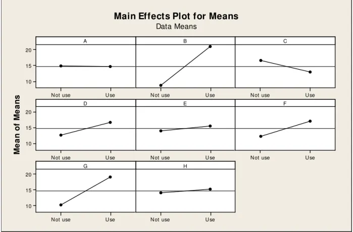
The factors with levels are given in Table 3 and the experimental layout is given in Table 4. The level averages (Phadke, 1989) and the effects (Montgomery, 2001) of factors are computed and are given in Table 5. The Table 5 showed that the factors namely, 25% (B), 60% (D), 80% (F) and 90 % (G) of TC execution have comparatively large effects on the response. The main effect plot given in Fig. 1 also confirmed the same result. The optimum combination of levels that will maximize S/N ratio is to use
these factors for calculating MD. Hence it is concluded that bug fix progress at 25%, 60%, 80% and
90% TC execution are the critical for differentiating the successful projects (normal group) from the unsuccessful projects (abnormal group). In other words, 25%, 60%, 80% and 90% TC execution are the critical milestones at which the bug fixing progress need to be controlled so that all the detected bugs can be fixed before the scheduled release of the software. Hence a control procedure is developed to quantitatively manage the bug fix progress at critical milestones during system testing phase.
U se N ot use
20
15
10
U se
N ot use N ot use U se
U se N ot use
20
15
10
U se
N ot use N ot use U se
U se N ot use
20
15
10
U se N ot use
A
M
e
a
n
o
f
M
e
a
n
s
B C
D E F
G H
Main Effects Plot for Means
Data Means
Fig. 1. Main Effect Plot
Table 3
Factors and Levels
SL No. Factor Name Factor Code Level 1 Level 2
1 10% TC Execution A Use Not Use
2 25% TC Execution B Use Not Use
3 50% TC Execution C Use Not Use
4 60% TC Execution D Use Not Use
5 70% TC Execution E Use Not Use
6 80% TC Execution F Use Not Use
7 90% TC Execution G Use Not Use
1086
Table 4
Experimental Layout
Exp No A B C D E F G H S/N
1 Use Not use Use Use Use Not use Not use Not use -1.1491
2 Use Not use Not use Use Not use Use Use Use 17.8366
3 Not use Use Use Use Not use Not use Not use Use 19.7881
4 Use Use Not use Not use Not use Use Not use Not use 20.9005
5 Not use Use Not use Not use Use Not use Use Use 20.914
6 Use Use Use Not use Not use Not use Use Not use 14.0056
7 Not use Not use Not use Use Not use Not use Use Not use 14.5866
8 Use Use Use Use Use Use Use Use 30.2777
9 Not use Not use Use Not use Use Use Use Not use 17.7098
10 Use Not use Not use Not use Use Not use Not use Use 6.24593
11 Not use Not use Use Not use Not use Use Not use Use -3.3076
12 Not use Use Not use Use Use Use Not use Not use 19.1194
Table 5
Level averages and factor effects
Factor
Level Averages
Effect Rank
Use Not Use
A 14.80 14.69 -0.12 8
B 8.65 20.83 12.18 1
C 16.60 12.89 -3.71 5
D 12.75 16.74 4.00 4
E 13.97 15.52 1.55 6
F 12.40 17.09 4.69 3
G 10.27 19.22 8.96 2
H 14.20 15.29 1.10 7
4. Bug fixing process management
The step by step details of the bug fixing process management procedure are as follows:
a. Develop a model to predict or classify whether the software can be released on time (all the detected bugs can be fixed on time) using the bug fix progress at critical milestones as control factors. The critical milestones are identified using MTS.
b. As the system testing reach different milestones (various % of TC execution) feed the value of bug fix progress to the model and predict whether the software can be released on time.
c. Based on the prediction if software cannot be released on time, then make necessary adjustments in the subsequent milestones so that ultimately software can be released on time. While predicting the outcome using the model at intermediate milestones, the average values of normal group (successful projects) can be used for the control factors at the subsequent milestones.
In this research, the model is developed using a machine learning technique namely K-nearest neighbour. The traditional classification techniques like logistic regression and linear discriminant functions are not used because in many cases, the factors may be correlated or the relation between dependant variable and control factors may not be linear. The k-Nearest Neighbour (k-NN) method provides a simple approach for calculating predictions for unknown observations. It calculates a prediction by looking at similar observations and uses some function of their response values to make the prediction (Myatt, 2007). The model using k-NN is developed using Rapid miner software. The model is evaluated using the following criteria, namely accuracy (% of correct predictions), classification error (% of incorrect predictions), precision (ratio of positives correctly classified to the total predicted positives), recall (ratio of positives correctly classified to total positive) and f measure
(2pr/(p+r), where p is precision and r is recall). The values of the performance criteria for the k-NN
Table 6
Model performance criteria
k-NN
Accuracy 100
Classification Error 0.00
Precision 100
Recall 100
f measure 100
The application of MTS has reduced the number of control points in the bug fixing process. Henceforth the managers need not rigorously monitor and control the bug fixing process throughout the system testing phase. Moreover the control procedure enables the managers to make mid course corrections to the subsequent milestones in case the bug fixing is not on track. This gives more options and flexibility to the managers for using the resources for bug fixing.
A methodology to control bug fixing process can be developed without the use of Mahalanobis Taguchi system approach also. The advantage of MTS is that it reduces the number of control points. Moreover when the proposed methodology is compared with those without MTS shows that performance of MTS based methodology is better than that of others. The comparison results are given in Table 7. The Table 7 once again shows that MTS is superior to neural networks (Bachy & Franke, 2015; Sahoo et al., 2015) with small samples.
Table 7
Comparison of MTS methodology with other techniques
With MTS Without MTS
k-NN k-NN Neural Networks
Accuracy 100.00 88.89 33.33
Classification Error 0.00 11.11 66.67
Precision 100.00 100.00 33.33
Recall 100.00 66.67 100.00
f measure 100.00 80.00 50.00
5.Validation
The proposed methodology is validated with eight new projects. Out of the eight, six are successful in releasing the software on time and the remaining two are unsuccessful. The validation data with results is given in Table 8. The Table 8 shows that the methodology correctly classified the six successful projects as successful and the two unsuccessful projects as unsuccessful. Hence the company decided to use the proposed methodology to monitor the bug fixing process during system testing phase of software development.
Table 8
Validation of Results
Project id
% of TC Executed
Actual Project Status Predicted Project Status
25% 60% 80% 90%
1 0.59 0.65 0.84 0.96 Successful Successful
2 0.58 0.64 0.85 0.95 Successful Successful
3 0.62 0.67 0.85 0.93 Successful Successful
4 0.64 0.68 0.86 0.97 Successful Successful
5 0.61 0.66 0.85 0.96 Successful Successful
6 0.4 0.65 0.76 0.82 Unsuccessful Unsuccessful
7 0.57 0.69 0.86 0.93 Successful Successful
1088
6. Conclusions
In this paper, the authors discussed a methodology for quantitatively manage the bug fixing process which would ensure the release of the software on time with full functionalities. The Mahalanobis-Taguchi system, a multidimensional pattern recognition method, is used to discriminate the successful software projects from the unsuccessful ones. Then using MTS and design of experiments, the critical milestones in system testing phase at which the bug fix progress need to be controlled and monitored are identified. Finally a model is developed to quantitatively manage the bug fixing process.
The values of the various evaluation criteria namely accuracy, classification error, precision, recall and f measure shows that the performance of the model is very good. The performance of the model is also compared with models without the application of MTS methodology. The comparison showed that the MTS based methodology is superior to that of others.
The application of MTS also reduced the number of control points for bug fixing processes during system testing. This provides the managers with more options and flexibility in utilization of resources for bug fixing. The proposed methodology also provide warnings as system testing is in progress and allows the managers to make mid-course corrections, if required, to achieve the desired goal of fixing all detected bugs on time and release the software as per schedule. The proposed methodology is also validated with eight new projects and results are very encouraging.
Acknowledgment
The authors are thankful to Prof. A K Chaudhuri, director, ADAAP process solutions and Mr. Shin Taguchi, president, ASI consulting group for their support and encouragement in carrying out this work.
References
Agrawal, M., & Chari, K. (2007). Software effort, quality, and cycle time: A study of CMM level 5 projects. IEEE Transactions on Software Engineering,33(3), 145-156.
Akhyar, G., Che Haron, C. H., & Ghani, J. A. (2008). Application of Taguchi method in the optimization of turning parameters for surface roughness. International Journal of Science
Engineering and Technology, l (3), 60 – 66.
Asada, M. (2001). Wafer yield prediction by the Mahalanobis-Taguchi system. IEEE International
Workshop on Statistical Methodology, 6, 25-28.
Bachy, B., & Franke, J. (2015). Modeling and optimization of laser direct structuring process using artificial neural network and response surface methodology. International Journal of Industrial
Engineering Computations, 6,553 - 564.
Berkani, S., Yallese, M.A., Boulanouar, L., & Mabrouki, T. (2015). Statistical analysis of AISI304 austenitic stainless steel machining using Ti(C, N)/Al2O3/TiN CVD coated carbide tool.
International Journal of Industrial Engineering Computations, 6,539 - 552.
Box, G. E., Hunter, W. G., & Hunter, S. J. (1978.) Statistics for Experiments: An Introduction to
Design, Data Analysis, and Model Building. Wiley, New York.
Chowdhury, K. K., & John, Boby. (2003). Optimization of the Induction Hardening Operation using Robust Design. Journal of Quality Engineering Forum,11(4), 70-76.
Cudney, E. A., Hong, J., Jugulum, R., Paryani, K., Ragsdell, K.M., & Taguchi, G. (2007). An Evaluation of Mahalanobis-Taguchi Systems and Neural Network for Multivariate Pattern Recognition. Journal of Industrial and System Engineering, 1(2), 139 – 150.
Cudney, E. A., Paryani, K., & Ragsdell, K. M. (2007). Applying the Mahalanobis-Taguchi system to vehicle ride. Journal of Industrial and System Engineering, 1(3), 251 – 259.
Fenton, N. E., & Pfleeger, S. L. (1996). Software Metrics, a rigours and practical approach. 2nd Edition, International Thomson Computer Press.
Fisher, R. A. (1974) The Design f Experiments. Hafner press, New York.
Fowlkes, W.Y., & Creveling, C.M. (1998). Engineering Methods for Robust Product Design –Using
Harter, D. E., Krishnan, M. S., & Slaughter, S. A. (2000). Effects of process maturity on quality, cycle time, and effort in software product development. Management Science, 46(4), 451-466.
Hayashi, S., Tanaka, Y., & Kodama, E. (2001). A new manufacturing control system using Mahalonobis distance for maximizing productivity. IEEE International Semiconductor
Manufacturing Symposium,15(4), 59 – 62.
Humphrey, W. S. (1988). Characterizing the software process: a maturity framework. IEEE Software, 5(2), 73-79.
Jacob, A.L., & Pillai, S.K. (2003). Statistical process control to improve coding and code review. IEEE
Software, 20(3), 50 – 55.
Jain, A. K., Robert, P. W. D., & Jianchang, M. (2000). Statistical pattern recognition: A review. IEEE
Transaction on Pattern Analysis and Machine Intelligence,22, 4-37.
Jalote, P. (2000). CMM in Practice: Process for Executing Software Projects at Infosys. Addison-Wesley.
Jiang, J. J., Klein, G., Hwang, H. G., Huang, J., & Hung, S. Y. (2004). An exploration of the relationship between software development process maturity and project performance. Information &
Management, 41(3), 279-288.
John, B., & Kadadevaramath, R. S. (2013). Optimization of the yield of a code review process.
Proceedings of the International Conference on Quality, Reliability and Operations Research, 161
– 168, Excel India Publishers. ISBN: 978-93-82880-27-1.
John, B.., & Kadadevaramath, R. S. (2014). A methodology for achieving the design review defect density goals in software development process. International Journal of Manufacturing, Industrial
& Management Engineering, 2(1), 181-191
John, B. (2014). Application of Mahalanobis-Taguchi system and design of experiments to reduce the field failures of splined shafts. International Journal of Quality & Reliability Management, 31(6), 681-697.
John, B. (2015). A dual response surface optimization methodology for achieving uniform coating thickness in powder coating process. International Journal of Industrial Engineering
Computations, 6, 469 – 480.
Jugulam, R., & Monplaisir, L. (2002). Comparison between Mahalanabis-Taguchi system and artificial neural networks. Journal of Quality Engineering Society, 10(1), 60-73.
Kacker, R.N. (1985). Off-line Quality Control, Parameter Design and Taguchi Method, Journal of
Quality Technology. 17, 176 – 209.
Mahalanobis, P.C. (1936). On Generalised distance in statistics. Proceedings of the National Institute
of Sciences of India, 2(1), 49–55.
Montgomery, D.C. (2001). Design and Analysis of Experiments. John Wiley & Sons, New York. Mishra, P.C., Das, D.K., Ukamanal, M., Routara, B.C., & Sahoo, A.K. (2015). Multi-response
optimization of process parameters using Taguchi method and grey relational analysis during turning AA 7075/SiC composite in dry and spray cooling environments. International Journal of
Industrial Engineering Computations, 6, 445 – 456.
Myatt, G. (2007). Making Sense of Data: A Practical Guide to Exploratory Data Analysis and Data
Mining, Vol. 1. John Wiley & Sons, Inc.
Naik, K., & Tripathy, P (2008). Software Testing and Quality Assurance. John Wiley and Sons. Perry, W. (1995). Effective Methods for Software Testing. John Wiley & Sons.
Phadke, M.S. (1989). Quality engineering using robust design. Prentice Hall, USA.
Raczynski, B., & Curtis, B. (2008). Software data violate SPC’s underlying assumptions. IEEE
Software, 25(3), 49.
Rama Rao, S., & Padmanabhan., G (2012). Application of Taguchi methods and ANOVA in optimization of process parameters for metal removal rate in electrochemical machining of Al/5%SiC composites. International Journal of Engineering Research and Applications, 2(3), 192 – 197.
1090
Sahoo, A. K., Rout, A. K., & Das, D. K. (2015). Response surface and artificial neural network prediction model and optimization for surface roughness in machining. International Journal of
Industrial Engineering Computations, 6, 229 – 240.
Taguchi, G., Chowdhury, S., & Wu, Y. (2001). The Mahalanobis-Taguchi System. McGraw Hill, New York.
Taguchi, G., & Rajesh, J. (2000). New Trends in Multivariate Diagnosis. Sankhya: Indian Journal of
Statistics, Series B, 62(2), 233-248.
Taguchi, G. (1980). Introduction to Off-line Quality Control. Central Japan Quality Control Association, Japan
Tian, J. (2005). Software Quality Engineering. John Wiley and Sons.
Weller, E., & Card, D. (2008). Applying SPC to software development: where and why. IEEE Software,
25(3), 48-50.
Woodall, W. H., Koulelik, R., Ysui, K. L., Kim, S. B., Stoumbos, Z. G., & Carvounis, C. P. (2003). A review and analysis of the Mahalanobis - Taguchi System. Technometrics, 45(1), 1- 30.
Wu, Y. (2004). Pattern Recognition Using Mahalanobis Distance. Journal of Quality Engineering