Annales Geophysicae (2003) 21: 1257–1261 cEuropean Geosciences Union 2003
Annales
Geophysicae
How did the solar wind structure change around the solar
maximum? From interplanetary scintillation observation
K. Fujiki1, M. Kojima1, M. Tokumaru1, T. Ohmi1, A. Yokobe1,*, K. Hayashi1, D. J. McComas2, and H. A. Elliott2
1Solar-Terrestrial Environment Laboratory, Nagoya University, 3-13 Honohara, Toyokawa, Aichi, Japan 2Southwest Research Institute, San Antonio, TX, USA
*SGI Japan, Ltd., 4-20-3 Ebisu, Shinjuku, Tokyo, Japan
Received: 9 September 2002 – Revised: 22 April 2002 – Accepted: 15 May 2003
Abstract. Observations from the second Ulysses fast lati-tude scan show that the global structure of solar wind near solar maximum is much more complex than at solar mini-mum. Soon after solar maximum, Ulysses observed a po-lar coronal hole (high speed) plasma with magnetic popo-larity of the new solar cycle in the Northern Hemisphere. We an-alyze the solar wind structure at and near solar maximum using interplanetary scintillation (IPS) measurements. To do this, we have developed a new tomographic technique, which improves our ability to examine the complex structure of the solar wind at solar maximum. Our IPS results show that in 1999 and 2000 the total area with speed greater than 700 km s−1 is significantly reduced first in the Northern
Hemisphere and then in the Southern Hemisphere. For year 2001, we find that the formation of large areas of fast so-lar wind around the north pole precedes the formation of large polar coronal holes around the southern pole by several months. The IPS observations show a high level agreement to the Ulysses observation, particularly in coronal holes. Key words. Interplanetary physics (solar wind plasma) – Radio science (remote sensing)
1 Introduction
The solar wind is generally well characterized by fast and slow regions (bimodal) around solar minimum, with the slow solar wind confined around the Sun’s streamer belt and the fast solar wind observed at higher latitudes (McComas et al., 1998). When solar activity increases, the low speed solar wind region extends to higher latitudes.
Ulysses observed the latitude structure of the solar wind at solar maximum with its second fast latitude scan (Novem-ber 2000–Octo(Novem-ber 2001). At this time a more complex solar wind structure was found compared to the simpler bimodal solar wind observed near solar minimum (McComas et al., Correspondence to:K. Fujiki
2002). Soon after solar maximum Ulysses again observed fast solar wind above 40◦N.
Ground-based interplanetary scintillation (IPS) observa-tions provide valuable estimates of the three-dimensional ve-locity structure of the inner heliosphere on a continuous ba-sis. We use the interplanetary scintillation observations of natural radio sources obtained with the Solar-Terrestrial En-vironment Laboratory system at Nagoya University in Japan. IPS signals of a natural radio source are affected by a bias, which is caused by a weighted integration along the line-of-sight. Solar wind speed is derived from the IPS signals using the Computer-Assisted Tomography (CAT) technique (Ko-jima et al., 1998), which removes the bias and improves spa-tial resolution. The CAT technique has been shown to work well around solar minimum. At solar minimum the bimodal velocity structure is reproduced well, and IPS CAT results agree well with Ulysses’ first fast latitude scan observations (e.g. Kojima et al., 1998, 2001). The tomographic analysis requires a stable solar wind velocity structure over one so-lar rotation, because all of the IPS data in a given Carrington rotation are used to produce a velocity map (V-map). Since the solar structure varies significantly over a solar rotation around solar maximum, the CAT method cannot produce an accurate V-map because the data are averaged over a long period of time. We introduce a modified version of the tomo-graphic technique that reduces the length of time averaged. We refer to this new technique as Time Series Tomography (TST). We then examine the variation of the solar wind ve-locity structure from 1998 (rising phase) to 2001 (after solar maximum), and compare our TST results with Ulysses solar maximum observations to test the validity of our technique.
2 Observation and analysis
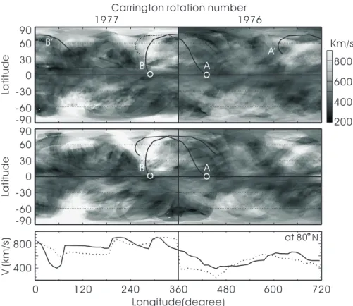
sen-Fig. 1.Typical example of the difference between original CAT and TST. Solid curve in top and middle panels are the line-of-sight of 3C119 observed in DOY 152(a)and DOY 162(b), respectively. White circles represent the position of the Earth each day. Longitudinal velocity profiles of original CAT (dotted) and TST (solid) at 80◦N are plotted in bottom panels.
sitive to the interplanetary scintillation observation. Obser-vations are obtained 8 h a day from each station, except dur-ing winter when heavy snow lies on a reflector of the anten-nas. As mentioned above, we employ the CAT procedure to reduce the line-of-sight integration effect. The original CAT produces a V-map using IPS data from a specific Car-rington rotation. Velocity data determined using IPS obser-vations are projected onto the source surface (2.5Rs) along Archimedean spiral. If there are enough line-of-sight cross-ings, the CAT produces a V-map with high accuracy. Fig-ure 1(a) shows original CAT results for CR 1976 and 1977. A V-map for each rotation is reconstructed independently and arranged. Solid curves are line-of-sight of 3C119 observed in DOY 152 (LOS-A) and 162 (LOS-B). LOS-A and LOS-B are assigned to CR 1976 and 1977, respectively. Then the LOS-A jumps to LOS-A’ after crossing the 360◦longitude. Longitudinal velocity profile at 80◦N latitude for the CAT map is plotted in Fig. 1c (dotted line). A large velocity jump is observed in 360◦longitude, and similar longitudinal dis-continuities are often seen in the boundaries of Carrington rotations during solar maximum. These structures are arti-facts which are caused by the projection method of the CAT procedure. In this method, the solar wind structure is as-sumed to be stable. Thus, the original CAT uses data that is distant in time, but close in longitude to create a V-map which is consistent with IPS observations when the large-scale structure of the solar wind was only changing slowly.
At solar maximum, the V-map obtained by using CAT is affected by averaging effects because the solar wind struc-ture varies rapidly. To reduce this effect we introduce a mod-ified tomographic technique-time-series tomography. In this method, line-of-sights are assigned to the neighboring Car-rington rotations and all of the line-of-sights obtained in a year are projected on a large, multi-rotation Carrington map (Fig. 2 and Fig. 3 upper panel). Figure 1b shows a part of TST map in 2001. LOS-A and -B are projected across the boundary of the line-of-sight. The solid curve in Fig. 1c shows a smooth variation of the solar wind velocity at the boundary of rotation period. The discrepancy between the original CAT and TST is only a mapping method of line-of-sight. Following an iterative fitting procedure, the process is identical to that employed in the CAT method. Original CAT and TST reconstructed almost the same V-map during the solar minimum when the solar wind velocity structure is stable (Ohmi PhD thesis, 2003). On the other hand, the TST method leads to much better results during the solar maxi-mum.
3 Results
K. Fujiki et al.: Solar wind structure change around the solar maximum 1259
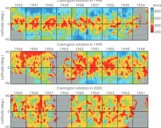
Fig. 2.Solar wind velocity structure around the solar maximum. Top to bottom panels show continuous variation of solar wind structure in the years from 1998 to 2000. Gray regions are data gap.
Fig. 3.Comparison between IPS and Ulysses observations. Velocity map in Carrington rotations from 1974 to 1981 are estimated from IPS observation. Coloured circle plots show Ulysses data which is traced back to 2.5Rs. The colour scale for the circle plots are same as the
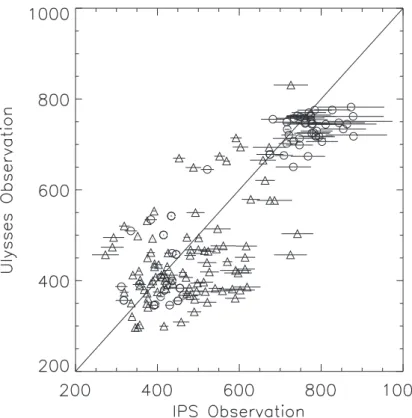
Fig. 4. Correlation between IPS and Ulysses observations. Triangle and cir-cle plots show the data at latitudes lower and higher than 45◦, respectively. Plots which did not converge are not in-cluded.
2000, we did not use data observed in November or Decem-ber of 2000 because it was not sufficient to reproduce the solar wind structure at high latitudes in the Southern Hemi-sphere where Ulysses passed during this period.
Figure 2 shows results of TST analysis for the year from 1998 (top panel) to 2000 (bottom panel). The velocity struc-ture in 1998 is still bimodal, and the fast solar wind around the north pole disappeared in CR 1951 (1999). However, the fast solar wind around the south pole is still observed in this year. Then the fast solar wind at high latitudes dis-appeared completely in 2000. Note that there is about a four-month gap between these maps because IPS observa-tions were stopped in the winter season due to heavy snow.
The upper panel of Fig. 3 shows a V-map from rotation 1974 (end-March) to 1981 (end-October) in year 2001. Near the end of July, powerful lightening unfortunately struck our observation system at the foot of Mt. Fuji. The electronic system was severely damaged and the observations stopped for about one month (gray region in CR 1979). The fast solar wind already appeared in CR 1974 at the north pole, local-ized in longitude (Fig. 3). The fast solar wind disappeared in CR 1975 and CR 1976 and appeared again in CR 1977. By CR 1980 the fast solar wind surrounded the north pole. At the south pole the fast solar wind appeared in CR 1977 and disappeared in CR 1980.
The circles in Fig. 3 indicate Ulysses observations with the same colour scale as the V-map. In this figure the Ulysses data has been ballistically mapped back to 2.5Rs using the observed solar wind speed. Gaps in the Ulysses data, like those at the boundary between CR 1977 and 1978, arise from
the large difference in observed solar wind speed. These gaps are always seen when Ulysses passes a boundary between fast and slow solar wind regions.
The lower panel in Fig. 3 provides a comparison between IPS and Ulysses data. Error bars for the tomographic analy-sis are shown. The rapid increase in the solar wind velocity that appeared in the low latitude around DOY 110 is a coro-nal mass ejection. Ulysses observed fast solar wind around DOY 170, 200, 220 and then reaches a fast solar wind region near the pole (CR 1980 and 1981). According to the Ulysses trajectory in the upper panel, it is clear that Ulysses passed near the boundary between fast and slow solar wind regions. On the other hand, the IPS and Ulysses data at low latitude where slow solar wind is observed do not correlate well with each other.
4 Summary and discussion
We employed time-series tomography to derive the solar wind velocity structure around solar maximum. We find that fast solar wind at the north pole disappeared in mid-1999 and at the south pole in 2000. Slow solar wind regions occupied almost all of the area on the source surface (2.5Rs) in this year. The recovery of the fast solar wind at the north pole precedes that at the south pole by a few solar rotations.
K. Fujiki et al.: Solar wind structure change around the solar maximum 1261 the boundary of the fast and slow solar wind regions.
Al-though we have no data for CR 1979, a localized fast so-lar wind region existed for three Carrington rotations (CR 1978–1979), since Ulysses observed fast solar wind at almost the same Carrington longitude in CR 1979. Thereafter, the fast solar wind region extends around the north pole in CR 1980. Differences between IPS and Ulysses observations in-creased in CR 1981. The velocities observed by IPS are near 900 km s−1, which is the upper limit in tomographic process to avoid divergence of the velocity, created by insufficient data coverage around the north pole.
Figure 4 shows the correlation between IPS and Ulysses observations. The high-latitude plots in CR 1981 are not include because they did not converge in the TST process. Latitudes higher than 45◦ (circles) are concentrated around the line. On the other hand, the data at the latitude lower than 45◦(triangles) are somewhat more scattered. One pos-sible reason is that the solar wind structure observed at the Ulysses position (1.4–2.0 AU) is significantly different from the structure observed by IPS (0.1–0.9 AU). The solar wind structure is gradually changed by stream-stream interaction. Another possible reason is that the V-map is temporary aver-aged because IPS data observed on different days is used in the TST reconstruction. The TST require about two weeks to deconvolve a specified position in the V-map. The pho-tospheric magnetic structure and shape of coronal streamer change rapidly in comparison with this length of time re-quired for TST analysis. Although the velocity structure can be reconstructed at low latitude with TST averaging of the data over time, differences between the TST V-map and Ulysses observations can be large at low latitudes or in low
solar wind speeds.
Acknowledgements. Topical Editor R. Forsyth thanks P. Liewer and another referee for their help in evaluating this paper.
References
McComas, D. J., Balogh, A., Bame, S. J., Barraclough, B. L., Feld-man, W. C., Forsyth, R., Goldstein, B. E., Gosling, J. T., Funsten, H. O., Neugebauer, M., Riley, P., and Skoug, R.: Ulysses’ return to the slow solar wind, Geophys. Res. Lett., 25, 1–4, 1998. McComas, D. J., Elliott, H. A., Gosling, J. T., Reisenfeld, D. B.,
Skoug, R. M., Goldstein, B. E., Neugebauer, M., and Balogh, A.: Ulysses’ second fast-latitude scan: Complexity near solar maximum and the reformation of polar coronal holes, Geophys. Res. Lett., 29(9), 10.1029/2001GL014164, 2002.
Kojima, M., Tokumaru, M., Watanabe, H., Yokobe, A., Asai, K., Jackson, B. V., and Hick, P. L.: Heliospheric tomography using interplanetary scintillation observations, 2, Latitude and helio-spheric distance dependence of solar wind structure at 0.1–1 AU, J. Geophys Res., 103, 1981–1989, 1998.
Kojima, M., Fujiki, K., Ohmi, T., Tokumaru, M., Yokobe, V., and Hakamada, K.: Latitudinal Velocity Structures up to the Solar Poles Estimated from IPS Tomography Analysis, J. Geophys. Res, 106, 15 677–15 686, 2001.
Kojima, M., Fujiki, K., Tokumaru, M., Ohmi, T., Shimizu, Y., Yokobe, A., Jackson, B. V., and Hick, P. L.: Tomographic Analysis of Solar Wind Structure Using Interplanetary Scin-tillation, COSPAR Colloquium Series, Vol. 12, 55–59, Proc. COSPAR Colloquium “Space Weather Study Using Multi-point Techniques”, 2002.