Implementation of a Neural Network Using Simulator and Petri Nets*

(1)

Implementation of a Neural Network Using Simulator

and Petri Nets*

Nayden Valkov Nenkov

Faculty of Mathematics and Informatics University of Shumen “Episkop Konstantin Preslavsky”

9700, Shumen, Bulgaria

Elitsa Zdravkova Spasova

Faculty of Mathematics and Informatics University of Shumen “Episkop Konstantin Preslavsky”

9700, Shumen, Bulgaria

Abstract—This paper describes construction of multilayer perceptron by open source neural networks simulator - Neuroph and Petri net. The described multilayer perceptron solves logical function "xor "- exclusive or. The aim is to explore the possibilities of description of the neural networks by Petri Nets. The selected neural network (multilayer perceptron) allows to be seen clearly the advantages and disadvantages of the realizing through simulator. The selected logical function does not have a linear separability. After consumption of a neural network on a simulator was investigated implementation by Petri Nets. The results are used to determine and to consider opportunities for different discrete representations of the same model and the same subject area.

Keywords—neural networks; simulators; logical or; petri net

I. INTRODUCTION

In the beginning we will examine Petri nets and their possible applications. In this paper we will emphasize precisely modeling power of Petri nets, as will examine their ability to present neural networks.

The simulator selected for implementation to the neural network in this study is NeuroPh, which is Java - based, object - oriented simulator. NeuroPh is also open-source and it offers many opportunities for different architectures of neural networks [8]. NeuroPh is lightweight frameworks allowed to simulate neural networks and can be use basic for the development of standard types of neural network architectures. It contains well designed open source library and a small number of core classes that correspond to basic concepts in neural networks. There is a good graphics editor to quickly build java - based components of neural networks.

One thing that makes Petri nets interesting is that they provide a balance between modeling power and analyzability: many things one would like to know about concurrent systems can be automatically determined for Petri nets, although some of those things are very expensive to determine in the general case. Several subclasses of Petri nets have been studied that can still model interesting classes of concurrent systems, while these problems become easier [1].

Since firing is nondeterministic, and multiple tokens may be present anywhere in the net (even in the same place), Petri nets are well suited for modeling the concurrent behavior of distributed systems [3, 7]. Petri nets are state-transition systems that extend a class of nets called elementary nets [5, 6]. Unless an execution policy is defined, the execution of Petri nets is

nondeterministic: when multiple transitions are enabled at the same time, any one of them may fire.

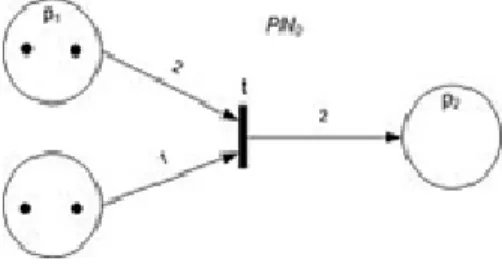
Fig. 1. Petri Net with an enabled transition

In the given diagram of a Petri net [3], the place circles may encompass more than one token to show the number of times a place appears in a configuration. The configuration of tokens distributed over an entire Petri net diagram is called amarking. In the diagram of a Petri net, places are conventionally depicted with circles, transitions with long narrow rectangles and arcs as one-way arrows that show connections of places to transitions or transitions to places. If the diagram were of an elementary net, then those places in a configuration would be conventionally depicted as circles, where each circle encompasses a single dot called atoken. Syntactically a Petri net is described by graph of the network. There is many alternative definitions. The following formal definition is loosely based on [2]. A Petri net graph (called Petri net by some, but see below) is a 3-tuple, (S, T, W) where

• S is a finite set of places • T is a finite set of transitions

• S and T are disjoint, i.e. no object can be both a place and a transition

W: (S × T) ∪ (T ×S) → N (1) is a multiset of arcs, i.e. it assigns to each arc a non-negative integer arc multiplicity (or weight); note that no arc may connect two places or two transitions.

Here, in this definition we have conditions mainly for sets S and T.

The flow relation is the set of arcs:

F = {(x, y)| W(x, y) >0} (2) In many textbooks, arcs can only have multiplicity 1. These texts often define Petri nets using F instead of W. When using

(2)

this convention, a Petri net graph is a bipartitemultigraph(S∪ T, F)with node partitions S and T.

The preset of a transition t is the set of its input places:

t = {s ∈ S | W(s, t) >0} (3) itspost set is the set of its output places:

t = {s ∈ S |W(t, s) >0} (4) Definitions of pre- and post-sets of places are analogous.

A marking of a Petri net (graph) is a multiset of its places, i.e., a mapping M: S→ ℕ .We say the marking assigns to each place a number of tokens.

Here we can introduce one more definition of Petri nets. As you can see, this definition is now based on the concept of graph of the network: A Petri net (called marked Petri net by some, see above) is a 4-tuple (S, T, W, M0), where

• (S, T, W) is a Petri net graph;

• M0 is the initial marking, a marking of the Petri net graph.

In words:

• firing a transition t in a marking M consumes W(s, t) tokens from each of its input places s, and produces

W(t, s) tokens in each of its output places s

• a transition is enabled (it may fire) in M if there are enough tokens in its input places for the consumptions to be possible [4]., i.e. if.

∀s: M(s) ≥ W(s, t) (5)

In this study first will be implemented neural network through simulator for neural networks and then will be used Petri nets. It has been made realization of a neural network of logical function exclusive or (XOR). This standard is a logical function which can be realized with NeuroPh and it is suitable for realization with Petri nets. This results from values, which suggests the logical function - 0 and 1. They are relatively simple and suitable for different types of presentations.

II. METHODOLOGY

In the beginning of the study we will realize neural network through neural network simulator. The neural network which we have choose for the study implemented a simple logical function “exclusive or”. This logical function is linearly inseparable. The neural network which we are building in this case is a multilayer perceptron. We choose this type of neural network, because linear inseparable function can be realized with a single-layer perceptron. Table 1 shows the essence of the logical operation “exclusive or”.

TABLE I. EXCLUSIVE OR

A B A XOR B

0 0 0

0 1 1

1 0 1

1 1 0

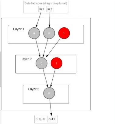
Commonly used artificial neural network simulators include theStuttgart Neural Network Simulator(SNNS), Emergent, JavaNNS, Neural LabandNetMaker. For this study is selected the simulator NeurophStudio. This simulator has the potential to realize the different algorithms for training neural networks and arbitrary architectures. This neural network implements logical operation “exclusive or”. There are two input neurons, one neuron in the hidden layer and one output neuron. Figure 3 shows a model of the neural network implemented on NeurophStudio. In this structure of the neural network is used some results from "Research of simulators for neural networks through the implementation of multilayer perceptron". [9].

Fig. 2. Neural network which realizes a logic operation XOR (simulatorNeurophStudio)

The training of the network is performed using the truth table of the logical operation ''exclusive or'', including following parameters:

Max error: 0.01

Learning rate: 0.2

It can be seen that the network is fully trained after 4000 iterations. After transferring this threshold begins a process of re-training and error begins to grow again.

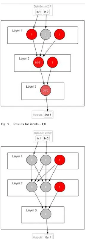
Once the network is trained, we ask sample inputs - 1; 1. At testing network with a sample input 1; 1 result is the following - the value of neuron in the hidden layer is 0,781; value of the neuron in the output layer is 0.263.

(3)

Fig. 3. Total Network Error Graph

Fig. 4. Results for inputs - 1;1

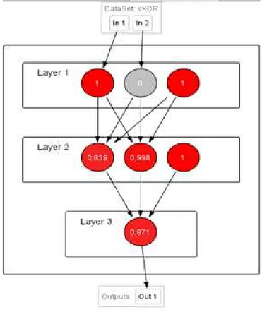
We testing network with a sample input 1; 0. The result is following - the value of neurons in the hidden layer is 0,839 and 0,998; value of the neuron in the output layer is 0.871.

This is shown in Figure 5.

We continue the study with another neural network. To see the difference in test cases, we will recreate the neural network by another type multilayer perceptron. This multilayer perceptron will decide the same task like the neural network above. The new neural network will have again one hidden layer, but with two neurons in it.

Figure 6 shows a model of a neural network implemented the same logical function. There are two input neurons, two neurons in the hidden layer and one output neuron.

Fig. 5. Results for inputs - 1;0

Fig. 6. Neural network, which realizes a logic operation XOR, including two neurons in hidden layer

It can be seen that the network is fully trained after 1900 iterations.

(4)

Fig. 7. Total Neural Network Graph

Fig. 8. Results for inputs - 1,1

We testing network with a sample input 1; 0. The result is following - the value of neurons in the hidden layer is 0,839 and 0,998; value of the neuron in the output layer is 0.871.

It can be seen that the results for the second architecture of the neural network are very good. This is particularly in the case when the neural network should give as a result 1. Thus we did tests of two input suit in the simulator for Neural Networks.

Fig. 9. Results for input - 1;0

We make a comparison between the graph in the simulator and the description of graph by Petri net. To create a graph of Petri nets we must define sets S, T, M0. Let's first of all to stick to the first model of the architecture of the neural network which has one neuron in the hidden layer. In this case the set S is consists of the input neuron, the neuron of the hidden layer and the output neuron. Especially for values in the set S we take an example pairs of logic function ''exclusive or'', two of which we already discussed in examples for simulator NeurophStudio. So far we have two values in this set. We added also and the output values - 0 or 1 for each example, as well as the value of a hidden neuron. The value of the hidden neuron is rather rounded. The set T consists of three connections between neurons - between the two input neurons and neurons of the hidden layer (2) and the connection between neurons of the hidden layer and the output neuron (1). The set Mo is the initial initialization of the neural network weights. To build a graph of Petri nets we consider also sets P. These sets contain specific examples and actually reflect the positive examples of T. This set contains a different number of elements for each example and includes input and output values which are equal to 1. This is actually 1 of the set T (excluding the value of the hidden neuron), which is subsequently recognized as a marker in the graph of Petri nets.

For the four cases of logical function can be built eight Petri nets:

(5)

Second: S - 0; 1; 0; 1

Mo - random initial weights of links T - Weights of links to specific iteration Set P2 - 1 element.

Third: S - 1; 0; 0; 1

Fourth: S - 1; 1; 0; 0

Mo - random initial weights of links T - Weights of links to specific iteration Set P4 - 2 elements.

Fifth: S - 0; 0; 1; 1

Sixth: S - 0; 1; 1; 1

Seventh: S - 1; 0; 1; 0

Eighth: S - 1; 1; 1; 0

Making a comparison between the two architectures of both established neural networks. Let us now discuss the case with the second architecture of the neural network. Here we have two neurons in the hidden layer. This means that the set S is increased by 1 unit, and multitudes T and M0 increased double. Therefore, there could be built 16 major Petri nets.

The first of them: S - 0; 0; 0; 0; 0 Mo - random initial weights of links T - Weights of links to specific iteration Set P1 - 0 elements.

Second: S - 0; 1; 0; 0;1

Third: S - 1; 0; 0; 0;1

Fourth: S - 1, 1, 0, 0, 0

Fifth: S - 0; 0; 1; 0; 1

Sixth: S - 0; 1; 1; 0; 1

Mo - random initial weights of links T - Weights of links to specific iteration

Set P6 - 2 elements. Seventh: S - 1; 0; 1; 0; 0

Eighth: S - 1; 1; 1; 0; 0

Ninth: S - 0; 0; 0; 1; 0

Tenth: S - 0; 1; 0; 1; 1

Eleven: S - 1; 0; 0; 1; 1

Twelve: S - 1; 1; 0; 1; 0

Thirteen: S - 0; 0; 1; 1; 1

Fourteen: S - 0; 1; 1; 1; 1

Fifteen: S - 1; 0; 1; 1; 0

Sixteenth: S - 1; 1; 1; 1; 0

In the case when the plurality of T have different values (0 and 1, 1 and 0) is obtained activation of the neuron of the output layer and the output is 1. In other cases, the output of the network is 0. This is actually case when neural network implements logical ''exclusive or'' function.

The sets T and Mo in Petri nets could give suggestion for the convergence of the network: how fast neural network will be trained, whether the training set is appropriate, how many test to be used, etc.

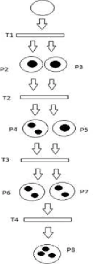
We can build a graph of the petri nets to the first example of architecture of the neural network.

(6)

determines the placement of a marker in these fields. From states P2 and P3 we already go to states P4 and P5. In fourth position, both input values are 1. We put two markers in the box. In the next state output value is 1, so we put a marker in the box. In the following two conditions P6 and P7 we have two markers in the fields. In them one input value and the output are 1. In the last state both inputs and outputs are 1. So we have three markers in this field.

We remind that this is research of the first neural network. In the same way can be examined case of the second neural network with two neurons in the hidden layer. Since it is identical we shall not dwell on it here in detail.

Fig. 10.Petri net for the first architecture of the neural network

Thus created graph of Petri nets can be very useful. Here the ability of Petri nets of analysis may be used. The research of fields can give many details on the neural network. Could be analyzed the truth in the result of the neural network. Neural network gives correct result where in the fields is missing marker or has two markers. In the study neural network we have the correct outcome in Example 1, 4, 6, 7 (here we look at sample values in set S). After building Petri nets based on these examples, we building a graph of the Petri net. And here we see that the fields corresponding to the correct result have two markers. It is possible in general there is no marker. So just looking the markers of graph of the petri nets can be seen how much truth there is neural network.

We see the ability the graph of the petri nets to be used to predict the accuracy of neural network. So using it can be selected at appropriate architecture of the neural network. It can be seen that Petri nets are very useful tool not only for the representation of neural networks, but also for their study.

III. CONCLUSION

The petri nets can be useful in determining the possible activations in the neural network and achievable conditions. The graph of Petri nets can follow all possible input examples of neural network. It can be seen where the neural network A

has a correct result and where - not. Thus, by displaying the authenticity of the result in the neural network could be found ways to improving it. There is the possibility of conducting research on different architectures of neural networks. The petri nets could help to find a suitable architecture of the neural network. The results can be very useful in training of the neural networks. By imaging the neural network through graph of Petri nets could be found on the appropriate input examples with which to be trained network. So can be significantly reduced training time. Just should be selected input examples with two markers in the graph (or without markers) of the Petri net. Training neural networks can be much facilitated. The results can be applied in lectures and education on neural networks. The study of specific architecture of the neural network can be examined with Petri nets. Here it can be determined which is the appropriate neural network for the specific subject area and the specific problem. Thus can predict which architecture of the neural network will be most suitable (how many layers, how many neurons).

Research in this area can be extended. Until now research has not included the algorithm for training the neural network. Remains to be seen how it can affect in Petri nets. What will show such inclusion, how it will be implemented and what is the results of it, is the subject of a future researches.

ACKNOWLEDGMENT

This article was published possible through support of the University of Shumen "Episkop Konstantin Preslavsky" and its program for development research project: „Study of intelligent methods and applications of simulators of neural networks and optimum methods of learning“.

REFERENCES

[1] Girault C., Valk R., Petri nets for systemengineering. guide to modeling, verification, and application, 2003, ISBN 978-3-662-05324-9

[2] Esparza, J. and Nielsen, M., Decidability issues for Petri nets - a survey. Bulletin of the EATCS, 1995, (Revised Ed.). Retrieved 2014-05-14. [3] Petri, C. A. and Reisig, W., Petri net. Scholarpedia 3 (4): 6477., 2008,

DOI:10.4249 /scholarpedia. 6477.

[4] Peterson, J. L. ,. Petri Net Theory and the Modeling of Systems. Prentice Hall., 1981, pp. 23-42, ISBN 0-13-661983-5

[5] Reisig, W., Understanding Petri nets. Modeling techniques, analysis methods, cese studies, 2013, ISBN 978-3-642-33278-4

[6] Reisig, W., Petri Nets and Algebraic Specifications. Theoretical Computer Science 80 (1), 1991, pp.1–34. DOI:10.1016/0304-3975(91)90203-e (references)

[7] Rozenburg, G. and Engelfriet, J.,. Elementary Net Systems. Lectures on Petri Nets I: Basic Models - Advances in Petri Nets. Lecture Notes in Computer Science 1491. Springer., 1998, pp. 12 –121.

[8] Sevarac, Z., Neuroph - Java neural network framework, Retrieved from http://neuroph.sourceforge.net/ ( May, 2012).