A high-order conservative collocation scheme and its application to global shallow-water equations

www.geosci-model-dev.net/8/221/2015/ doi:10.5194/gmd-8-221-2015

© Author(s) 2015. CC Attribution 3.0 License.

A high-order conservative collocation scheme and its application to

global shallow-water equations

C. Chen1, X. Li2, X. Shen2, and F. Xiao3

1_{School of Human Settlement and Civil Engineering, Xi’an Jiaotong University, Xi’an, China} 2_{Center of Numerical Weather Prediction, China Meteorological Administration, Beijing, China} 3_{Department of Energy Sciences, Tokyo Institute of Technology, Yokohama, Japan}

Correspondence to:C. Chen (cgchen@mail.xjtu.edu.cn)

Received: 31 May 2014 – Published in Geosci. Model Dev. Discuss.: 10 July 2014 Revised: 20 November 2014 – Accepted: 8 January 2015 – Published: 10 February 2015

Abstract. In this paper, an efficient and conservative col-location method is proposed and used to develop a global shallow-water model. Being a nodal type high-order scheme, the present method solves the pointwise values of dependent variables as the unknowns within each control volume. The solution points are arranged as Gauss–Legendre points to achieve high-order accuracy. The time evolution equations to update the unknowns are derived under the flux reconstruc-tion (FR) framework (Huynh, 2007). Constraint condireconstruc-tions used to build the spatial reconstruction for the flux function include the pointwise values of flux function at the solution points, which are computed directly from the dependent vari-ables, as well as the numerical fluxes at the boundaries of the computational element, which are obtained as Riemann solu-tions between the adjacent elements. Given the reconstructed flux function, the time tendencies of the unknowns can be obtained directly from the governing equations of differen-tial form. The resulting schemes have super convergence and rigorous numerical conservativeness.

A three-point scheme of fifth-order accuracy is presented and analyzed in this paper. The proposed scheme is adopted to develop the global shallow-water model on the cubed-sphere grid, where the local high-order reconstruction is very beneficial for the data communications between adja-cent patches. We have used the standard benchmark tests to verify the numerical model, which reveals its great potential as a candidate formulation for developing high-performance general circulation models.

1 Introduction

A recent trend in developing global models for atmospheric and oceanic general circulations is the increasing use of the high-order schemes that make use of local reconstructions and have the so-called spectral convergence. Among many others are those reported in Giraldo et al. (2002), Thomas and Loft (2005), Giraldo and Warburton (2005), Nair et al. (2005a, b), Taylor and Fournier (2010) and Blaise and St-Cyr (2012). Two major advantages that make these models attractive are (1) they can reach the targeted numerical ac-curacy more quickly by increasing the number of degrees of freedom (DOFs) (or unknowns), and (2) they can be more computationally intensive with respect to the data communi-cations in parallel processing (Dennis et al., 2012).

(2013) that the flux reconstruction can be implemented in a more flexible way, and other new schemes can be generated by properly choosing different types of constraint conditions. In this paper, we introduce a new scheme which is differ-ent from the existing nodal DG and SE methods under the FR framework. The scheme, the so-called Gauss–Legendre-point-based conservative collocation (GLPCC) method, is a kind of collocation method that solves the governing equa-tions of differential form at the solution points, and is very simple and easy to follow. The Fourier analysis and the nu-merical tests show that the present scheme has the same super convergence property as the DG method. A global shallow-water equation (SWE) model has been developed by imple-menting the three-point GLPCC scheme on a cubed-sphere grid. The model has been verified by the benchmark tests. The numerical results show the fifth-order accuracy of the present global SWE model. All the numerical outputs look favorably comparable to other existing methods.

The rest of this paper is organized as follows. In Sect. 2, the numerical formulations in a one-dimensional case are de-scribed in detail. The extension of the proposed scheme to a global shallow-water model on a cubed-sphere grid is dis-cussed in Sect. 3. In Sect. 4, several widely used benchmark tests are solved by the proposed model to verify its perfor-mance in comparison with other existing models. Finally, the Conclusion is given in Sect. 5.

2 Numerical formulations

2.1 Scheme in one-dimensional scalar case

The first-order scalar hyperbolic conservation law in one di-mension is solved in this subsection:

∂q

∂t +

∂f (q)

∂x =0, (1)

whereqis a dependent variable andf a flux function. The computational domain,x_{∈ [}xl, xr], is divided intoI elements with the grid spacing of1xi=x_i+1

2−xi−

1 2 for the ith elementC_{i :} h_x

i−12, xi+ 1 2 i

.

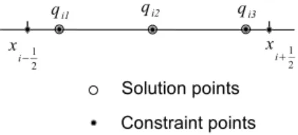
The computational variables (unknowns) are defined at several solution points within each element, e.g., within el-ementC_{ithe point values,qim(m=1,2, . . ., M), are defined}

at the solution points (xim). High-order schemes can be built by increasing the number of the solution points. In this pa-per, we describe the GLPCC scheme that has three solution points for each grid element (M₌3). The configuration of local degrees of freedom is shown in Fig. 1 by the hollow circles. To achieve the best accuracy, the DOFs are arranged at Gauss–Legendre points in this study:

xi1=xi−

√

3

2√51xi, xi2=xi andxi3=xi+

√

3

2√51xi, (2) wherexi is the center of the elementxi=(x_i−1

2+xi+12)/2.

Figure 1.Configuration of DOFs and constraint conditions in a one-dimensional case.

The unknowns are updated by applying the differential-form governing equations (Eq. 1) at solution points as

∂qim

∂t = −

∂f (q)

∂x

im

. (3)

As a result, the key task left is to evaluate the derivatives of the flux function, which is realized by reconstructing the piecewise polynomial for flux function,F_i(x), over each el-ement. Once the reconstructed flux function is obtained, the derivative of flux function is approximated by

∂f (q)

∂x

im

≈

∂F_i(x)

∂x

im

. (4)

In Huynh (2007), FR is formulated by two correction func-tions which assure the continuity at the two cell boundaries and collocate with the so-called primary Lagrange recon-struction at their zero points. Therefore, the existing nodal type schemes can be recast under the FR framework with different correction functions. In Xiao et al. (2013), a more general FR framework was proposed by introducing multi-moment constraint conditions including nodal values, first-order derivatives and even second-first-order derivatives to de-termine the flux reconstruction. Here, we will develop a new method to reconstruct the flux function, which is more straightforward and simpler compared with the methods dis-cussed in either Huynh (2007) or Xiao et al. (2013).

We assume that the reconstructed flux function over theith element,F_i(x), has the form of

F_{i(x)=ci0+ci1(x−xi)+ci2(x−xi)}2

+ci3(x−xi)3+ci4(x−xi)4, (5)

where the coefficients,ci0, ci1, . . ., ci4, are determined by a collocation method, which meets five constraint conditions specified at five constraint points (shown in Fig. 1 by the solid circles) as

      

F_i(xim) =f (qim) , m=1 to 3

F_ix_i

−12

=fe_i

−12

F_ix_i

+12

=fe_i

+12

, (6)

wherefe_i

±12 are the values of flux function at the cell

In Eq. (6),f (qim)are calculated by three known DOFs at solution points. The values of flux function at the boundaries are obtained by solving the Riemann problems with the val-ues of dependent variables interpolated separately from two adjacent elements. Considering the interface atx_i

−12, we get

two values of flux function from elementsC_i−1andC_ias

fL

i−12 = f

qL

i−12

=f

h

Qi−1

x_i−1

2 i

and

fR

i−12 = f

qR

i−12

=fhQi

x_i

−12 i

, (7)

where Qi(x) is a spatial reconstruction for the dependent variable based on local DOFs, having the form of

Qi(x)=

3

X

m₌1

L_m(x)qim

, (8)

where the Lagrange basis function L_m(x)=

Q3

s=1,s6=m x−xis

xim−xis.

Then the numerical fluxfe_i−1

2 at the boundary is obtained

by an approximate Riemann solver as

e

f_i

−12 =

1 2

fL

i−12 +

fR

i−12

+1

2a

qL

i−12−

qR

i−12

, (9)

wherea₌ f′ qavg

i−12

withf′(q)=∂f (q)∂q being the charac-teristic speed. A simple averagingqavg

i₋1₂ = qL

i−12

+qR

i−12

2 is used in the present paper.

Based on the Riemann solver at cell boundaries, the pro-posed scheme is essentially an upwind type method. As a result, the inherent numerical dissipation is included and sta-bilizes the numerical solutions. We did not use any extra arti-ficial viscosity in the shallow-water model for the numerical tests presented in the paper.

It is easy to show that the proposed scheme is conservative in terms of the volume-integrated average of each element:

q_i=

3

X

m=1

(wimqim) , (10)

where the weightswim are obtained by integrating the La-grange basis function as

wim=

1

1xi

x

i+1₂ Z

x

i−1₂

L_{m(x)dx, (11)}

and are exactly the same as those in Gaussian quadrature of degree 5.

A direct proof of this observation is obtained by integrat-ing Eq. (3) over the grid element, yieldintegrat-ing the followintegrat-ing con-servative formulation:

∂

∂t 1xiqi

=1xi

3

X

m=1

wim ∂qim ∂t = − e f_i

+12− e

f_i

−12

, (12)

where1xiqi is the total mass within the elementCi. With the above spatial discretization, the Runge–Kutta method is used to solve the following semi-discrete equation (ODE):

dqim dt =D(q

∗_{), (13)}

whereD_{represents the spatial discretization and} q∗ is the dependent variables known at timet₌t∗.

A fifth-order Runge–Kutta scheme (Fehlberg, 1958) is adopted in the numerical tests to examine the convergence rate:

qim t∗+1t=qim∗

+1t

17 144d1+

25 36d3+

1 72d4−

25 72d5+

25 48d6

, (14) where                         

d1 =D(q∗)

d2 =D

q∗₊1₅1t d1

d3 =D

q∗₊2 51t d2

d4 =D

q∗₊9 41t d1+

15

41t d2−51t d3

d5 =D

q∗₋ 63 1001t d1+

9 51t d2−

13 201t d3+

2 251t d4

d6 =D

q∗₋ 6 251t d1+

4 51t d2+

2 151t d3+

8 751t d4

. (15)

In other cases, a third-order scheme (Shu, 1988) is adopted to reduce the computational cost, which does not noticeably degrade the numerical accuracy since the truncation errors of the spatial discretization are usually dominant. It is written as

qim t∗+1t=qim∗ +1t

1 6d1+

1 6d2+

2 3d3

, (16) where       

d1= D(q∗)

d2= D(q∗+1t d1)

d3= D

q∗₊1₄1t d1+1₄1t d2

. (17)

2.2 Spectral analysis and convergence test

We conduct the spectral analysis (Huynh, 2007; Xiao et al., 2013) to theoretically study the performance of the GLPCC scheme by considering the following linear equation

∂q

∂t +

∂q

This linear equation is discretized on an uniform grid with

1x₌1. Since the advection speed is positive, the spatial dis-cretization for the three DOFs defined in elementC_iinvolves

the six DOFs within elementsC_{i and}C_{i−1and can be written}

as the following linear combination as

∂qim

∂t = −

_∂q

∂x

im

=

3

X

s=1

ebmsqi−1,s+

3

X

s=1

(bmsqis) , (19)

whereebms andbms are the coefficients for the DOFs within elementsC_i−1andC_{i, respectively, which can be obtained by}

applying the proposed scheme to governing equation Eq. (18) in elementC_ias

e

b11=1,eb12= −4δ−2,eb13= −

2δ₊1 2δ₋1,

e

b21= −

1

4δ₊2,eb22=1,eb23= 1 4δ₋2,

e

b31= −

2δ₋1

2δ₊1,eb32=4δ−2,eb33=1, (20) and

b11=

4δ2₊8δ₋3 2δ (2δ₋1) , b12=

4δ2₊2δ₋2

δ , b13= −

2δ₋1 2δ ,

b21=

δ₋1

2δ (2δ₋1), b22= −1, b23= −

δ₊1

2δ (2δ₊1),

b31= −

2δ₊1 2δ , b32=

−4δ2₊2δ₊2

δ ,

b33=

4δ2₋8δ₋3

2δ (2δ₊1) , (21)

with the parameterδ₌

√

3 2√5.

With a wave solution of q (x, t )₌eIω(x+t ) (I₌√_−1),

we have

qi−1,m=e−Iω1xqim=e−Iωqim. (22)

Above spatial discretization can be simplified as

∂qim

∂t = −

∂q ∂x

im

=

3

X

s=1

(Bmsqis) and

Bms=

ebmse−Iω+bms

. (23)

Considering the all of DOFs in elementC_{i, a matrix-form}

spatial discretization formulation is obtained as

∂q_i

∂t =Bqi, (24)

whereq_{i= [}qi1, qi2, qi3]T and the components of the 3×3 matrixBare coefficientsBms (m=1 to 3,s=1 to 3).

−12 −10 −8 −6 −4 −2 0

−8 −6 −4 −2 0 2 4 6 8

Re

Im

Figure 2.The spectrum of the semi-discrete scheme.

With the wave solution, the exact expression for the spatial discretization of Eq. (18) is

∂q_i

∂t = −Iωqi. (25)

The numerical property of the proposed scheme can be ex-amined by analyzing the eigenvalues of matrixBin Eq. (24). Truncation errors of the spatial discretization are computed by comparing the principal eigenvalues of matrixBand its exact solution −I_{ω, and the convergence rate can be}

Table 1.Numerical errors at two wave numbers and corresponding convergence rate.

Wave number ω=π₈ ω=π₄ Order

Error −3.1408×10−5−4.2715×10−6i −5.0466×10−7−3.4068×10−8i 4.97

0 1 2 3 4 5 6

−4 −3.5 −3 −2.5 −2 −1.5 −1 −0.5 0 0.5 1

ω

Re(S(

ω

))

Exact

0 1 2 3 4 5 6

0 1 2 3 4 5 6 7 8

ω

Im(S(

ω

))

Exact

Figure 3.Numerical dispersion (left) and dissipation (right) rela-tions of the semi-discrete scheme.

uses constraint conditions on the point values, first- and second-order derivatives of flux functions at the cell bound-aries where Riemann solvers in terms of derivatives of the flux function are required. Compared with the DG3 scheme, the proposed scheme is easier to be implemented and thus has less computational overheads. Though the MCV5 scheme gives better spectra (eigenvalues are closer to imaginary) than the DG3 scheme and the present scheme, it adopts more DOFs under the same grid spacing, i.e., 4I₊1 DOFs for MCV5 and 3I DOFs for DG3 and the present scheme, whereI is the total number of elements. Both MCV5 and the present scheme show slightly higher numerical frequency in the high wave number regime, which is commonly observed in other spectral-convergence schemes, such as DG. Consid-ering the results of the spectral analysis, the proposed scheme is a very competitive framework to build high-order schemes compared with existing advanced methods.

Advection of a smooth sine wave is then computed by the GLPCC scheme on a series of refined uniform grids to nu-merically checking the converge rate. The test case is spec-ified by solving Eq. (18) with initial condition q(x,0)₌

sin(2π x)and periodical boundary condition overx_{∈ [}0,1]. A CFL number of 0.1 is adopted in this example. Nor-malizedl1,l2andl∞errors and corresponding convergence

rate are given in Table 2. Again, the fifth-order convergence is obtained, which agrees with the conclusion in the above spectral analysis.

2.3 Extension to system of equations

The proposed scheme is then extended to a hyperbolic sys-tem withLequations in one dimension, which is written as

∂q

∂t +

∂f(q)

∂x =0, (26)

whereqis the vector of dependent variables andf the vector of flux functions.

Above formulations can be directly applied to each equa-tion of the hyperbolic system, except that the Riemann prob-lem, which is required at the cell boundaries between dif-ferent elements to determine the values of flux functions, is solved for a coupled system of equations.

For a hyperbolic system of equations, the approximate Riemann solver used at interfacex_i

−12 is obtained by

rewrit-ing Eq. (9) as

f_i

−12 =

1 2

fL

i−12+

fR

i−12

+1

2a

qL

i−12 −

qR

i−12

, (27)

where the vectorsfL

i−12

,fR

i−12

,qL i−12

andqR i−12

are evaluated by applying the formulations designed for scalar case to each component of the vector. In this paper, we use a simple ap-proximate Riemann solver, the local Lax–Friedrichs (LLF) solver, whereais reduced to a positive real number as

a₌max(_|λ1|,|λ2|, . . .,|λL|) , (28)

whereλl (l=1 toL)are eigenvalues of matrixA

qavg

i−12

,

withA(q)₌∂f_∂q(q) andqavg

i−12 =

qL i₋1

2

+qR i₋1

2

2 .

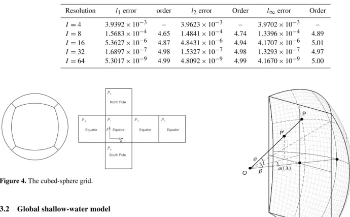
3 Global shallow-water model on cubed-sphere grid 3.1 Cubed-sphere grid

Table 2.Numerical errors and convergence rates for advection of a sine wave.

Resolution l1error order l2error Order l∞error Order

I=4 3.9392×10−3 – 3.9623×10−3 – 3.9702×10−3 –

I=8 1.5683×10−4 4.65 1.4841×10−4 4.74 1.3396×10−4 4.89

I=16 5.3627×10−6 4.87 4.8431×10−6 4.94 4.1707×10−6 5.01

I=32 1.6897×10−7 4.98 1.5327×10−7 4.98 1.3293×10−7 4.97

I₌64 5.3017_×10−9 4.99 4.8092_×10−9 4.99 4.1670_×10−9 5.00

Figure 4.The cubed-sphere grid.

3.2 Global shallow-water model

The local curvilinear coordinate system (ξ, η) is shown in Fig. 5, whereP is a point on sphere surface, andP′is corre-sponding point on the cube surface through a gnomonic pro-jection. λandθ represent the longitude and latitude.αand

β are central angles spanning from₋π₄ toπ₄ for each patch. Local coordinates are defined byξ₌Rαandη₌Rβwhere

Ris the radius of the Earth.

To build a high-order global model, the governing equa-tions are rewritten onto the general curvilinear coordinates. As a result, the numerical schemes developed for Carte-sian grid are straightforwardly applied in the computational space. The shallow-water equations are recast on each spher-ical patch in flux form as

∂q

∂t +

∂e(q)

∂ξ +

∂f(q)

∂η =s(q) , (29)

where dependent variables are q₌h√Gh, u, viT with water depth h, covariant velocity vector (u, v) and Ja-cobian of transformation √G; flux vectors are e₌

h_√

Gh_eu, g (h₊hs)+1₂(euu+evv) ,0

iT

in ξ direction and

f ₌h√Gh_ev,0, g (h₊hs)+1₂(euu+evv)

iT

in η direction with gravitational accelerationg, height of the bottom moun-tainhs and contravariant velocity vector(eu,ev); source term

is s₌h0, √G_ev (f₊ζ ) , ₋√G_eu (f₊ζ )iT with Coriolis

parameter f ₌2sinθ; rotation speed of the Earth ₌

7.292×10−5s−1and relative vorticityζ ₌√1

G

∂v ∂ξ −

∂u ∂η

.

Figure 5.The gnomonic projection.

The expression of metric tensorGij can be found in Nair et al. (2005a, b). Jacobian of the transformation is√G₌ q

det Gij

and the covariant and the contravariant velocity components are connected through

eu

ev

=Gij

u v

, (30)

whereGij₌ Gij−1.

Here, taking√Ghas the model variable assures the global conservation of total mass, and the total height is used in the flux term. Consequently, the proposed model can easily deal with the topographic source term in a balanced way (Xing and Shu, 2005).

The numerical formulations for a two-dimensional scheme are easily obtained under the present framework by imple-menting the one-dimensional GLPCC formulations inξ and

ηdirections respectively as

_∂q

∂t

=

_∂q

∂t

ξ

+

_∂q

∂t

η

+s, (31)

Figure 6.Configuration of DOFs and constraint conditions in a two-dimensional case.

_∂q

∂t

ξ

= −∂e(q)_∂ξ and

_∂q

∂t

η

= −∂f_∂η(q) (32)

are discretized along the grid lines inξ andηdirections. We describe the numerical procedure in ξ direction here as follows. Inη direction, similar procedure is adopted for spatial discretization by simply exchanging e and ξ with

f and η. Considering three DOFs, i.e., q_ij1nk, q_ij2nk and

q_ij3nk, along the nth row (n₌1 to 3) of element C_{ij k=} h

ξ_i−1

2, ξi+ 1 2 i

× h

η_j−1

2, ηj+

1 2 i

on patchk(defined at solution points denoted by the hollow circles in Fig. 6), we have the task to discretize the following equations:

_∂q

ij mnk

∂t

ξ

= −

_∂e

∂ξ

ij mnk

. (33)

As in a one-dimensional case, a fourth-order polynomial

E_{ij nk(x)is built for spatial reconstructions of flux functions} eto calculate the derivative ofewith regard toξ as

_∂e

∂ξ

ij mnk

=

_∂E

ij nk(ξ )

∂ξ

ij mnk

, (34)

whereE(ξ )can be obtained by applying the constraint con-ditions at five constraint points (solid circles in Fig. 6) along the nth row of elementC_{ij k, which are pointwise values of}

flux functionseincluding three from DOFs directly and other two by solving Riemann problems along thenth rows of the adjacent elements.

The LLF approximate Riemann solver is adopted. It means that the parameter a in Eq. (27) reads a_{= |e}u_{| +}pG11_gh. Details of solving the Riemann problem in a global shallow-water model using governing equations Eq. (29) can be re-ferred to in Nair et al. (2005b).

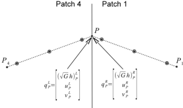
How to set up the boundary conditions along the twelve patch boundaries is a key problem to construct a global

Figure 7.The Riemann problem along patch boundary edge be-tween patch 1 and 4.

model on cubed-sphere grid. With enough information from the adjacent patch, above numerical formulations can be applied on each patch independently. In the present study, the values of dependent variables are required to be inter-polated from the grid lines in the adjacent patch, for ex-ample, as shown in Fig. 7 for the boundary edge between patch 1 and patch 4. When we solve the Riemann problem at point P on patch 1, qR_P=√GhR

P, u R p, vPR

T

is ob-tained by interpolation along the grid line P P1. Whereas,

qL_{P =}√GhL

P, u L p, vLP

T

need to be interpolated from the DOFs defined along grid lineP4P on patch 4. Since the co-ordinates on patch 1 and patch 4 are discontinuous at point

P, the values of the covariant velocity vector on the coor-dinate system on patch 4 should be projected to coorcoor-dinate system on patch 1 and the values of the scalar can be adopted directly. In comparison with our previous study (Chen and Xiao, 2008), in present the study we solve the Riemann prob-lem at patch boundary only in the direction perpendicular to the edge. The parameterain Eq. (27) is determined by the contravariant velocity component perpendicular to the edge and the water depth, which is exactly the same in two ad-jacent coordinate systems, since the water depth is a scalar independent of the coordinate system and the basis vector perpendicular to the edge is continuous between adjacent patches. As a result, solving the Riemann problem obtains the same result wherever the numerical procedure is con-ducted on patch 1 or patch 4. So, no additional corrections are required and the global conservation is guaranteed auto-matically.

4 Numerical tests

shallow--0.04

-0.04 -0.04

-0 .04 0.04

-0.04

-0.04 -0.04

-0.04

-0 .04 -0

.04

-0.04 -0.04

-0 .04

-0.0 4

-0.04

-0.04

-0.04

-0.04 -0

.04 -0.04

0 .08 0.08

0

.0

8

0 45 90 135 180 225 270 315 360

-9 0 -6 0 -3 0 0 30 60 90

1250

12 50

1250

1450

1

4

5

0

1450 1450

1650

165 0

1650

1650

1650

1850

1850

1850

18 50

1850

1850

2050

2050 2050

2050 20

50

225

2250

2250 22

50

2250

2250

22 50 2250

2450

2450 2450

2450

2450 24

50

2650

2650 26

50

2650

2650

2650

26 50 2650

2850

2850

285 0

2850

285 0 28

50 2850

0 45 90 135 180 225 270 315 360

-9 0 -6 0 -3 0 0 30 60 90

-0.04

-0.04 -0.04

-0.04

-0 .0

4

-0.04

-0.04 -0.04

-0.04 -0.04 -0.04 -0.04

-0 .0 4

-0.0 4

-0 .04

-0.04

-0.04

-0 .04 -0.04

-0.04

-0.0 4 -0

.04

-0.04 -0.04 -0.04

-0 .04

0.08

0.08

0.08 0.08

0 45 90 135 180 225 270 315 360

-9 0 -6 0 -3 0 0 30 60 90

1250 1250

1250 1250

1450 1450

1450 1450

1650 1650

1650 1650

1850 1850

1850 1850

2050 2050

2050

2250

2250 2250

2450 2450

2450 2450

2650 2650

2650 2650

2850 2850

2850 2850

0 45 90 135 180 225 270 315 360

-9 0 -6 0 -3 0 0 30 60 90

Figure 8.Numerical results and absolute errors of water depth for case 2 on gridG₁₂at day 5. Shown are water depth (top left) and absolute

error (top right) of the flow withγ=0 and water depth (bottom left) and absolute error (bottom right) of the flow withγ= π₄.

Table 3.Numerical errors and convergence rates for case 2 of the flow withγ=π₄.

Grid l1error l1order l2error l2order l∞error l∞order

G6 3.394×10−5 – 5.492×10−5 – 1.868×10−4 – G12 1.440×10−6 4.56 2.321×10−6 4.56 8.924×10−6 4.39 G24 5.367×10−8 4.75 8.317×10−8 4.80 3.457×10−7 4.69 G48 1.942×10−9 4.79 2.957×10−9 4.81 1.487×10−8 4.54

water model. All measurements of errors are defined follow-ing Williamson et al. (1992).

4.1 Williamson’s standard case 2: steady-state geostrophic flow

A balanced initial condition is specified in this case by using a height field as

gh₌gh0− Ru0+

u2₀

2

!

·(₋cosλcosθsinγ₊sinθcosγ )2, (35)

wheregh0=2.94×104,u0=2π R/(12 days) and the pa-rameterγ represents the angle between the rotation axis and polar axis of the Earth, and a velocity field (velocity compo-nents in longitude–latitude griduλanduθ) as

(

uλ =u0(cosθcosγ+sinθcosλsinγ )

uθ = −u0sinλsinγ

. (36)

As a result, both height and velocity fields should keep un-changing during integration. Additionally, the height field in this test case is considerably smooth. Thus, we run this test on a series of refined grids to check the convergence rate of

GLPCC global model. The results ofl1,l2andl∞errors and

convergence rates are given in Table 3. After extending the proposed high-order scheme to the spheric geometry through the application of the cubed-sphere grid, the original fifth-order accuracy as shown in one-dimensional simulations and spectral analysis is preserved in this test. Numerical results of height fields and absolute errors are shown in Fig. 8 for tests on gridG12, which means there are 12 elements in bothξand

5050

5050

5150 5150

515

5150

5250 5250

5250

5250

5250

5250 ₅₂₅₀

5350

5350

535 0 5350

350

5450 5450

5 4 50

5450

5550 5550

5550

555 0 5550

5650

5650 5650

5650 5650

5750 57

50 5750

5750

5750

5750

5850 5850

5850

5850

5

950

0 45 90 135 180 225 270 315 360

-9 0 -6 0 -3 0 0 30 60 90

5050 5050

5050 5050

5150 5150

5150

5150

5250 5250

5250

5350

5350

535 5350

5350

5450

5450 5450

5550 5550

55 50

5550

565 5650

56 50

5650

5650

5750 5750

57 50

5750

5850 5850

5850 5850

59 50 5950

0 45 90 135 180 225 270 315 360

-9 0 -6 0 -3 0 0 30 60 90

5050 5050

5050

5150

5150

51 50

5150

5250

5250

5250 5250

5350

5350

5350

5350

5450 5450

5450

5450

5450

5550 5550

5550

5550

5550

5650 5650

5650

565 0

5650

5750

57 50

5750

5750

5850

5850

5850 5850

5950

5950

0 45 90 135 180 225 270 315 360

-9 0 -6 0 -3 0 0 30 60 90

Figure 9.Numerical results of total height field for case 5 on gridG12at day 5 (top left), day 10 (top right) and day 15 (bottom).

0 5 10 15

−2 −1 0 1

2x 10

−15

DAY

Total Mass Error

Figure 10.Normalized conservation error of total mass on gridG12

for case 5.

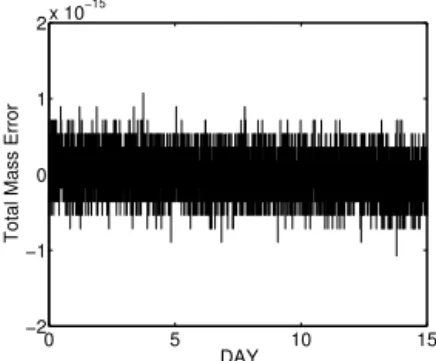
4.2 Williamson’s standard case 5: zonal flow over an isolated mountain

The total height and velocity field in this case is same as the above case 2 withγ₌0, excepth0=5960 m andu0= 20 m s−1_{. A bottom mountain is specified as}

hs=hs0

1₋ r

r0

, (37)

where hs0=2000 m, r0=π₉ and r=

minhr0,

p

(λ₋λc)2+(θ−θc)2

i

.

This test is adopted to check the performance of a shallow-water model to deal with a topographic source term. We run this test on a series of refined grids G6,G12,G24 andG48. Numerical results of height fields are shown in Fig. 9 for the total height field of the test on grids G12 at day 5, 10 and 15, which agree well with the spectral transform solutions on T213 grid (Jakob-Chien et al., 1995). Furthermore, the oscillations occurring at the boundary of the bottom moun-tain observed in spectral transform solutions are completely

0 5 10 15

10−10

10−8

10−6

10−4

10−2

100

Day

Enstrophy Error

G₆

G

12

G₂₄

G₄₈

0 5 10 15

10−10

10−8

10−6

10−4

10−2

Day

Total Energy Error

G₆

G

12

G₂₄

G₄₈

Figure 11.Normalized conservation errors of total energy and po-tential enstrophy on refined grids for case 5.

removed through a numerical treatment which balances the numerical flux and topographic source term (Chen and Xiao, 2008). The numerical results on finer grids are not depicted here since they are visibly identical to the results shown in Fig. 9. Present model assures the rigorous conservation of the total mass as shown in Fig. 10. The conservation errors of total energy and enstrophy are of particular interest for eval-uating the numerical dissipation of the model. As shown in Fig. 11, the conservation errors for total energy (left panel) and potential enstrophy (right panel) of tests on a series of refined grids are checked. As in the above case, to compare with our former fourth-order model this test case is checked on gridG20having the similar DOFs as the former 32×32×6 grid. The conservation errors are₋9.288_×10−7for total en-ergy and₋1.388_×10−5 for potential enstrophy and much smaller than those by fourth-order model in Chen and Xiao (2008).

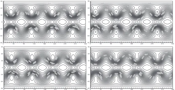
4.3 Williamson’s standard case 6: Rossby–Haurwitz wave

8300 8300 8300 8500 8500 8500

8500 8500 85

0 0 85 00 8 5 0 0

8700

8

70

0

8700 8700

8700

8700

8700 8700

8700 8 70 0 89 00 8900 8

900 8900

8 900

89 00 8900

890

0 8900

8900

9100

9100

9100

9100

91 00 910

0 910

0 9100

9300 9300

9300 930

0

9300 9300

9300 9300

9300

95 00 950

0 9500

9500

9500 9500

9500 9500

9700 9700

9700 9700

9700 9700

9700 9700

99 00 9900

9900 9900

9900 99

00 9900

10100 1010 0 1010 0 101 00

1010

0 101

00 10100

10300

1030

0 1030 0 103 00 1030 0 103 00

10500 10500

10 500

105 00

0 45 90 135 180 225 270 315 360

-9 0 -6 0 -3 0 0 30 60 90 8300 8300 8300 8300 8500 8500 8500 8500 8 5 0 0

8500

8500

8500

85

00 850

0

8

500

87 00 87

00

8 700

8700 8700

870 0 8 7 0 0 8700

870

0

8700

89 00 8900 890

0 8900

8900

8900 8900 8900

8900 89

00

9 100

9100

9100

91 00 9100

9100

9100

9100

9100

9100

9300 930

0 930 0 9300 93 00

9300 9300

93 00 9300

9500

950

0 9500

9500

9500 9500

9500 9500 9700 9700 9700 9700

9700 9700

9700 9700

9900 99 00 990 0 99 00 9900 9900 9900 9900

10100 101

00

1010

0

10100

10100 1010

0

10100 10100

10 300 10

30 0

10300 103

00

1030

0 10₃₀₀

10 30

0 10

500

10500

0 45 90 135 180 225 270 315 360

-9 0 -6 0 -3 0 0 30 60 90 8300 8300 8300 8500 8500 8500 8500

8500 850

0

8500

8500

8

5

00

8500

8700

8 7 00 87 00 8700 8700

8700 87

00 8700

87 00

870

0

8900 8900 8900

8900 8900

8900

89 0 0 8900

8900 890

0 9100 910 0 91 00 9100

9100

9100 9100

9100

91 00 910 0 9300 93₀₀

9300 930

0

93 00 9300

9300 9300

9500 9500

9500 9500 9500 9500 9500 950 0 9700 9700 9700 9700

9700 970 0 970 0 970 0

9900 9900

99 00 9900

9900 99 00 99 00 1010 0 1010 0 10100 1010 0

10100

10100

10100 1

0300 10300 103

00 10300

10 300

10 300 103

00 1030

0 10

500

0 45 90 135 180 225 270 315 360

-9 0 -6 0 -3 0 0 30 60 90 8300 8300 8300 8500 8500 8 5 0 0

8500 850

0 8 5 0 0 8500 8500 8500 8 5 00 8 700

870

0 8700

8700 870

0 8700 87 00 8 7 00 8700

8700

8900 8900

8900

8900

8900

8900

8900

890 0 8900

9100 9100

910

0 9100

910 0 9100

9100 9100

9100

93 00 930

0 9300

9300

9300 9300

9300 9300

9500 9500

9500 950 0 9500 950 0 950 0 95 00 970 0 9700

97 00 970 0 9700 9700 9700 9700

9900

9900 9900 9900 99 00 9900 9900 9900 10 100 10100 10100

10100

10100 10100 10 100 10 100 10 3₀₀ 103 00 10₃₀₀ 103 00 10 300 10 30 0 10 30 0 105 00 10 500

1050

0 10

5 00

0 45 90 135 180 225 270 315 360

-9 0 -6 0 -3 0 0 30 60 90

Figure 12.Numerical results of water depth for case 6 on gridG12at day 7 (top left), day 14 (top right) and on gridG24at day 7 (bottom

left) and day 14 (bottom right).

0 7 14

−2 −1 0 1

2x 10

−15

DAY

Total Mass Error

Figure 13.Normalized conservation error of total mass on gridG12

for case 6.

high-order schemes are always preferred to better capture the evolution of small scales. The spectral transform solution on fine T213 grid given by Jakob-Chien et al. (1995) is widely accepted as the reference solution to this test due to its good capability to reproduce the behavior of small scales. Numer-ical results of height fields by the GLPCC model are shown in Fig. 12 for tests on grids G12 andG24 at day 7 and 14. At day 7, no obvious difference is observed between the so-lutions on different grids and both agree well with the refer-ence solution. At day 14, obvious differrefer-ences are found on different grids. Eight circles of 8500 m exist in the results on the coarser grid G12, which are also found in the spec-tral transform solution on the T42 grid, but not in the results on the finer gridG24 by the GLPCC model and the spectral transform solutions on the T63 and T213 grids. Additionally, the contour lines of 8100 m exist in spectral transform solu-tion on the T213 grid, but not in present results and spectral transform solutions on the T42 and T63 grids. According to the analysis in Thuburn and Li (2000), this is due to the less

0 7 14

10−10 10−8 10−6 10−4 10−2 Day

Total Energy Error

G₆

G₁₂

G₂₄

G48

0 7 14

10−10 10−8 10−6 10−4 10−2 100 Day Enstrophy Error G₆ G12 G₂₄ G₄₈

Figure 14.Normalized conservation errors of total energy and po-tential enstrophy on refined grids for case 6.

inherent numerical viscosity on finer grids. As in case 5, to-tal mass is conserved to the machine precision as shown in Fig. 13 and the conservation errors for total energy and po-tential enstrophy are given in Fig. 14 for tests with different resolutions. Total energy error of₋6.131_×10−6and poten-tial enstrophy error of−1.032×10−3 are obtained by the present model running on gridG20, which are smaller than those obtained by our fourth-order model on the 32×32×6 grid (Chen and Xiao, 2008). This test was also checked in Chen et al. (2014a) by a third-order model (see their Fig. 19c and d), where many more DOFs (9 times more than those on gridG24) are adopted to obtain a result without eight circles of 8500 m at day 14. It reveals a well-accepted observation that a model of higher order converges faster to the reference solution, and should be more desirable in the atmospheric modeling.

4.4 Barotropic instability

Figure 15.Numerical results of water depth for balanced setup of

barotropic instability test on two gridsG24 (left) andG72(right).

Contour lines vary from 9000 to 10 100 m.

0 1 2 3 4 5

10−4 10−3

Day

l1

error

G₂₄ G

72

Figure 16.Normalizedl₁error of water depth for balanced setup of barotropic instability test on two grids.

The balanced setup is same as Williamson’s standard case 2, except the water depth changes with much larger gradient within a very narrow belt zone. This test is of special interest for global models on the cubed-sphere grid, since that nar-row belt zone is located along the boundary edges between patch 5 and patches 1, 2, 3 and 4. Extra numerical errors near boundary edges would easily pollute the numerical results. In practice, four-wave pattern errors may dominate the simu-lations on the coarse grids. For this case, we run the proposed model on a series of refined grids. By checking the conver-gence of the numerical results, we can figure out if the extra numerical errors generated by discontinuous coordinates can be suppressed by the proposed models with the increasing resolution. The unbalanced setup introduces a small pertur-bation to the height field. Thus, the balanced condition can not be preserved and the flow will evolve to a very complex pattern. Exact solution does not exist for unbalanced setup and a spectral transform solution on the T341 grid to this case given in Galewsky et al. (2004) at day 6 is adopted as reference solution. The details of setup of this test can be re-ferred to Galewsky et al. (2004).

4.4.1 Balanced setup

We test the balanced setup at first. The proposed model runs on two grids with different resolutions ofG24andG72. Nu-merical results of water depth after integrating for 5 days are

Figure 17.Numerical results of relative vorticity for unbalanced setup of barotropic instability test on a series of refined grids.

Con-tour lines vary from−1.1×10−4to−0.1×10−4by dashed lines

and 0.1_×10−4to 1.5_×10−4by solid lines.

shown in Fig. 15 and evolution of normalized l1 errors of water depth of two simulations are depicted in Fig. 16. On a coarse grid withG24, the numerical result is dominated by four-wave pattern errors and the balanced condition can not be preserved in simulation. The accuracy is obviously im-proved by increasing the resolution using gridG72. The nu-merical result of height field at day 5 is visually identical to the initial condition. The improvement of the accuracy can be also proven by checking the velocity componentuθ. Nu-merical results ofuθ, which stay at zero in exact solution, vary within a range of_±31 m s−1 _{on gridG}

24 and a much smaller range of_±0.8 m s−1 _{on gridG}

72. This test is more challenging for a cubed-sphere grid than other quasi-uniform spherical grids, e.g., a yin–yang grid or icosahedral grid. As shown in Fig. 16, at the very beginning of the simulation the

l1errors increase to a magnitude of about 10−4on coarse grid

4.4.2 Unbalanced setup

We run the unbalanced setup on a series of refined grids to check if the numerical result will converge to the reference solution on refined grids. Numerical results for relative vor-ticity field after integrating the proposed model for 6 days are shown in Fig. 17. Shown are the results on four grids with gradually refined resolutions ofG24,G48,G72andG96. On gridG24, the structure of numerical result is very differ-ent from the reference solution. After refining the grid res-olution, the result is improved on grid G48; except for the structure in top-left corner, it looks very similar to the refer-ence solution. On gridG72andG96, numerical results agree with the reference solution very well and there is no obvi-ous difference between these two contour plots. Compared with the results of our former fourth-order model, the con-tour lines look slightly less smooth. Similar results are found in the spectral transform reference solution. Since this test contains more significant gradients in the solution, a high-order scheme might need some extra numerical dissipation to remove the noise around the large gradients. Increasing the grid solution can effectively reduce the magnitude of the oscillations as shown in the present simulation.

5 Conclusions

In this paper, a three-point high-order GLPCC scheme is proposed under the framework of flux reconstruction. Three local DOFs are defined within each element at Gauss– Legendre points and a super convergence of fifth order is achieved. This single-cell-based method shares advantages with the DG and SE methods, such as high-order accuracy, grid flexibility, global conservation and high scalability for parallel processing. Meanwhile, it is much simpler and eas-ier to implement. With the application of the cubed-sphere grid, the global shallow-water model has been constructed using the GLPCC scheme. Benchmark tests are checked by using the present model, and promising results reveal that it is a potential framework to develop high-performance general circulation models for atmospheric and oceanic dynamics. As any high-order numerical scheme, additional dissipation or limiter projection might be needed in simulations of real case applications. Because of the algorithmic similarity, the existing works on high-order limiting projection and artificial dissipation devised for DG or SE methods are applicable to the GLPCC without substantial difficulty. Also future studies should focus on designing more reliable limiting projection formulations for the GLPCC and other FR schemes, which are able to deal with discontinuities without losing the over-all high-order accuracy.

Acknowledgements. This study is supported by the National Key

Technology R&D Program of China (grant no. 2012BAC22B01), the National Natural Science Foundation of China (grant nos.

11372242 and 41375108), and in part by the Japan Society for the promotion of Science (JSPS KAKENHI 24560187).

Edited by: L. Gross

References

Blaise, S. and St-Cyr, A.: A dynamic hp-adaptive discontinuous Galerkin method for shallow water flows on the sphere with ap-plication to a global tsunami simulation, Mon. Weather Rev., 140, 978–996, 2012.

Chen, C. G. and Xiao, F.: Shallow water model on cubed-sphere by multi-moment finite volume method, J. Comput. Phys., 227, 5019–5044, 2008.

Chen, C. G., Li, X. L., Shen, X. S., and Xiao, F.: Global shal-low water models based on multi-moment constrained finite vol-ume method and three quasi-uniform spherical grids, J. Comput. Phys., 271, 191–223, 2014a.

Chen, C. G., Bin, J. Z., Xiao, F., Li, X. L., and Shen, X. S.: Shal-low water model on cubed-sphere by multi-moment finite vol-ume method, Q. J. Roy. Meteorol. Soc., 140, 639–650, 2014b. Cockburn, B., Karniadakis, G., and Shu, C. (Eds.):

Discontinu-ous Galerkin Methods: Theory, Computation and Applications, Vol. 11 of Lecture Notes Lecture Notes in Computational Sci-ence and Engineering, Springer, 1st Edn., 2000.

Dennis, J., Edwards, J., Evans, K., Guba, O., Lauritzen, P., Mirin, A., St-Cyr, A., Taylor, M., and Worley, P.: CAM-SE: a scalable spectral element dynamical core for the community at-mosphere model, Int. J. High Perform. C., 26, 74–89, 2012. Fehlberg, E.: Eine Methode zur Fehlerverkleinerung beim

Runge-Kutta-Verfahren, Zeitschrift für Angewandte Mathematik und Mechanik, 38, 421–426, 1958.

Galewsky, J., Scott, R. K., and Polvani, L. M.: An initial-value prob-lem for testing numerical models of the global shallow-water equations, Tellus, 56, 429–440, 2004.

Giraldo, F. X. and Warburton, T.: A nodal triangle-based spectral element method for the shallow water equations on the sphere, J. Comput. Phys., 207, 129–150, 2005.

Giraldo, F. X., Hesthaven, J. S., and Warburton, T.: Nodal high-order discontinuous Galerkin methods for the spherical shallow water equations, J. Comput. Phys., 181, 499–525, 2002. Hesthaven, J. and Warburton, T.: Nodal Discontinuous Galerkin

Methods: Algorithms, Analysis, and Applications, Springer, 2008.

Huynh, H. T.: A flux reconstruction approach to high-order schemes including discontinuous Galerkin methods 2007-4079, 2007, AIAA Paper, 2007.

Ii, S. and Xiao, F.: High order multi-moment constrained finite vol-ume method. Part I: Basic formulation, J. Comput. Phys., 228, 3669–3707, 2009.

Ii, S. and Xiao, F.: A global shallow water model using high order multi-moment constrained finite volume method and icosahedral grid, J. Comput. Phys., 229, 1774–1796, 2010.

Jakob-Chien, R., Hack, J. J., and Williamson, D. L.: Spectral trans-form solutions to the shallow water test set, J. Comput. Phys., 119, 164–187, 1995.

Li, X. L. Chen, D. H., Peng, X. D., Takahashi, K., and Xiao, F.: A multimoment finite-volume shallow-water model on the Yin-Yang overset spherical grid, Mon. Weather Rev., 136, 3066– 3086, 2008.

Nair, R. D., Thomas, S. J., and Loft, R. D.: A discontinuous Galerkin transport scheme on the cubed sphere, Mon. Weather Rev., 133, 827–841, 2005a.

Nair, R. D., Thomas, S. J., and Loft, R. D.: A discontinuous Galerkin global shallow water model, Mon. Weather Rev., 133, 876–887, 2005b.

Patera, A.: A spectral element method for fluid dynamics: Lami-nar flow in a channel expansion, J. Comput. Phys., 54, 468–488, 1984.

Rancic, M., Purser, R. J., and Mesinger, F.: A global shallow-water model using an expanded spherical cube: gnomonic versus con-formal coordinates, Q. J. Roy. Meteorol. Soc., 122, 959–982, 1996.

Sadourny, R.: Conservative finite-difference approximations of the primitive equations on quasi-uniform spherical grids, Mon. Weather Rev., 100, 136–144, 1972.

Shu, C.-W.: Total-variation-diminishing time discretizations, SIAM J. Sci. Stat. Comput., 9, 1073–1084, 1988.

Taylor, M. A. and Fournier, A.: A compatible and conservative spec-tral element method on unstructured grids, J. Comput. Phys., 229, 5879–5895, 2010.

Thomas, S. and Loft, R.: The NCAR spectral element climate dy-namical core: semi-implicit Eulerian formulation, J. Sci. Com-put., 25, 307–322, 2005.

Thuburn, J. and Li, Y.: Numericial simulations of Rossby-Haurwitz waves, Tellus A, 52, 181–189, 2000.

Williamson, D. L., Drake, J. B., Hack, J. J., Jakob, R., and Swarz-trauber, P. N.: A standard test set for numerical approximations to the shallow water equations in spherical geometry, J. Comput. Phys., 102, 211–224, 1992.

Xiao, F., Ii, S., Chen, C., and Li, X.: A note on the general multi-moment constrained flux reconstruction formulation for high or-der schemes, Appl. Math. Model., 37, 5092–5108, 2013. Xing, Y. and Shu, C.-W.: High order finite difference WENO