Abstract
This paper focuses on analysis in determining the behaviour of vari-able amplitude strain signals based on extraction of segments. The constant Amplitude loading (CAL), that was used in the laboratory tests, was designed according to the variable amplitude loading (VAL) from Society of Automotive Engineers (SAE). The SAE strain signal was then edited to obtain those segments that cause fatigue damage to components. The segments were then sorted according to their amplitude and were used as a reference in the design of the CAL loading for the laboratory tests. The strain signals that were obtained from the laboratory tests were then analysed using fatigue life prediction approach and statistics, i.e. Weibull distribution anal-ysis. Based on the plots of the Probability Density Function (PDF), Cumulative Distribution Function (CDF) and the probability of fail-ure in the Weibull distribution analysis, it was shown that more than 70% failure occurred when the number of cycles approached 1.0 x 10¹¹. Therefore, the Weibull distribution analysis can be used as an alternative to predict the failure probability.
Keywords
Fatigue, signal processing, strain signal, variable amplitude, Weibull distribution
Probability Analysis in Determining the Behaviour of Variable
Amplitude Strain Signal Based on Extraction Segments
1 INTRODUCTION
Fatigue failure is a frequent phenomenon in industries, especially in the automotive field. According to a study by Gupta et al. (2006), the material damage caused by the phenomenon of fatigue results in major degradation in the structure. Early detection of fatigue damage is very important because continuous damage can result in catastrophic failure that will lead to components destruction and
M. F. M. Yunoh a
S. Abdullah b, *
M. H. M. Saad c
Z. M. Nopiah d
M. Z. Nuawi e
a Department of Mechanical and Materials
Engineering, Faculty of Engineering & Built Enviroment, Universiti Kebangsaan Malaysia, 43600 UKM Bangi, Selangor, Malaysia. [email protected]
b [email protected] c [email protected]; d [email protected]; e [email protected]
* Corresponding author: S. Abdullah, [email protected]
http://dx.doi.org/10.1590/1679-78254036
probably the loss of life. This failure could happen even though most of the properties of metal alloys have been thoroughly researched (Colin and Peter, 2009). Currently, various methods and tools have been developed to detect and reduce fatigue failure such as cracks and fractures.
Most of the common methods used are concerned with laboratory tests, data collection and anal-ysis using specific software (Lee and Han, 2009; Tsapi and soh, 2015). The field of signal processing in the analysis of fatigue data has attracted the interest of researchers until today. The prediction of fatigue life should be studied with an actual load to ensure a more accurate analysis. Therefore, in determining the fatigue life of automotive components, the actual loading must be used as the input data for the analysis of fatigue to obtain highly accurate results for the study (Wang et al. 1995). However, it is very expensive and time consuming to conduct the study in a real situation.
In actual applications, most of the engineering components are exposed to variable amplitude loading (VAL) that lead to failure and eventually cause cracks to appear (Wei et al. 2002; Mansor et al. 2017). The characterisation of fatigue life on materials is mostly done under a constant amplitude loading (CAL) to facilitate the analysis with existing equipment (Post et al. 2008). Hence, a method is needed to convert the VAL loading to a CAL loading that has almost the equivalent degree of fatigue damage. In this paper, the process of editing the strain signals obtained in real situations was used to design a constant signal that can be used in laboratory experiments to obtain the same results. The main focus of this paper was to predict the fatigue life of materials through laboratory tests and analyses using the Weibull distribution analysis.
2 THEORETICAL BACKGROUND
The Wavelet Transform is a method for summarising the data or functions that are operating in different frequencies. Wavelet Transform is widely used to study signals where the resolution is rela-tive to the scale that is providing the information in both domains of time and frequency (Wu & Liu, 2007). Wavelet Transform can be classified as Continuous Wavelet Transform (CWT) and Discrete Wavelet Transform (DWT). Until now, Wavelet Transform analysis is being used extensively in the field of engineering such as data compression, signal processing, image processing, as well as in the medical field (Sifuzzaman et al. 2009). Piotrkowski et al. (2009) used the Wavelet Transform appli-cation in acoustic emissions to detect damage and corrosion, while Chang and Chen (2005) used the Wavelet Transform to detect the position and depth of cracks in beams. Discrete Wavelet transform can be defined as in Equation (1):
dt nb t a a
t x n m
W ( , ) ( ) 0m2 *( 0m, 0)
(1)
where a represents the scale, and b, the time that is discretised from the continuous wavelet according to aa0m,bna0nb0,m and n are integers and b ≠ 0 is the translation step.
fixed expression, where it is merely stated as a failure whenever a small crack is detected (Stephens et al. 2001).
The strain life model that is commonly used in the prediction is the Coffin-Manson model. This model can provide a traditional prediction when the history of the compression load time is more influence and the mean stress is zero. This model can be defined by Equation (2):
c f f b f f
a N N
E (2 ) (2 )
' '
(2)
Two other models are usually used in experiments involving the mean stress effect, namely the Morrow and Smith Watson Topper (SWT) models. The Morrow model involves modifying the elastic strain part in the strain-life curve by taking into account the mean stress. This model is suitable for studying steel materials and predicting the fatigue life by taking into account the strain amplitude.
cf f b f f m f
a N N
E 1 (2 ) 2
' ' ' (3)
The parameter of damage that takes into account the maximum stress and the strain amplitude of a cycle for the SWT model can be expressed by Equation (4):
c b f f f b f f mak
a N N
E
' 2(2 )2
'
' (2 )
(4)In terms of the statistical analysis used in the field of engineering, the Weibull distribution is a theoretical model that has been used successfully. Through this model, the general distribution can be modelled within the range of the life distribution (Sivapragash et al., 2008). The Weibull distribu-tion is also suitable to study a failure analysis of a small number of samples. In this study, the 2-P Weibull distribution is shown in the following Equation (5):
x x
x
f ( : , ) exp (5)
In this study, f (x: θ: β) is the fatigue life probability that is equal to or less than θ, β, which are the scale perimeter and shape perimeter, respectively.
3 METHODOLOGIES
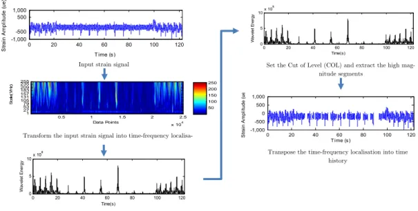
Figure 1: Process flow diagram of Wavelet Transform based on fatigue data editing method.
The maintained segments were then compiled and classified according to five categories, namely from the lowest to the highest strain amplitude. The strain amplitude values derived from all five categories were calculated to stress values by using the Ramberg-Osgood equation. This process is important for the design of the CAL loading, which must be based on the stress values. The Ramberg– Osgood equation was created to describe the nonlinear relationship between stress and strain. It is especially useful for metals that harden with plastic and showing a smooth elastic-plastic transition. The Ramberg-Osgood can be expressed by Equation (6):
n K
E E
(6)
Where, K and n are constants that depend on the material being considered.
The process flow in Figure 2 further shows the process for the conversion of the strain to stress. The equivalent damage can be used to construct the CAL loading from the actual VAL loading. This approach was used by changing the VAL loading to CAL loading based on the equivalent fatigue damage.
Fatigue tests were conducted on an SAE 5160 specimen, which is the material usually used for coil springs. In research, the sample of a material that is being tested must represents the mass of the material being studied, i.e. it must comprise the same source and undergo the same process. The SAE 5160 is categorised as a carbon steel material based on the designation issued by the SAE. The materials properties for SAE 5160 are tabulated in Table 1. In this laboratory test, the specimen, in the form of a sheet, was used in the experiment on fatigue under CAL loading. The dimensions for this specimen were according to the ASTM 606-92 standards. Usually, in monotonic stress and fatigue life experiments, round-shaped specimens are used. However, sheet specimens can also be used but these should be polished to eliminate the effects of machining (Lee et al., 2005). Figure 3 shows the completed specimen for fatigue test.
Input strain signal
Data Points Sc al e( 1/ H z)
0.5 1 1.5 2 2.5
x 104 1 27 53 79 105 131 157 183 209 235 255 50 100 150 200 250
Transform the input strain signal into time-frequency
localisa-0 20 40 60 80 100 120
0 5 10x 10
8 Time(s) W av el et E ne rg y
Transpose into time-frequency magnitude distribution
0 20 40 60 80 100 120
0 5 10x 10
8 Time(s) W av elet E ner gy
Set the Cut of Level (COL) and extract the high mag-nitude segments
Transpose the time-frequency localisation into time history
0 20 40 60 80 100 120
-1,000 500 -500 1,000 Time (s) S tra in A m pl itude (ue)
0 20 40 60 80 100 120
Figure 2: Flowchart of the conversion from strain to stress.
Properties Value
Ultimate tensile strength, Su (MPa) 1584
Modulus of elasticity, E (GPa) 207
Fatigue strength coefficient, σ’f (MPa) 2063
Fatigue strength exponent, b -0.08
Fatigue ductility exponent, c -1.05
Table 1: Mechanical properties for SAE 5160
Figure 3: Specimen in the form of a sheet that was used in the stress and fatigue test. Start
ɛ≥ɛ˳
Read the original strain amplitude, ɛ˳
Give an initial of stress, σ=1
Substitute the stress value into Ramberg-Osgood equation to get the strain value, ɛ
Compare the calculate strain value, ɛ with the original strain value, ɛ˳
The stress value equal to original strain value
σ = σ + 1
End
No
An accelerated fatigue test was conducted using a servo-hydraulic Instron 8874 machine with a capacity of ± 25 kN. Five specimens were used to obtain the mechanical properties under different CAL loadings. Each specimen was placed with a strain gauge to record the strain signal while the test was being conducted. Figure 4 shows the position of the specimen in the machine and the con-nection of the strain gauge to the data acquisition tool. In this experiment, the applied loads were 0.62 N, 1.2 N, 1.72 N, 3.68 N and 5.56 N. These load values were obtained based on the stress derived from the conversion of the strain amplitude using the Ramberg-Osgood equation. In this experiment, a frequency of 10 Hz was used.
Figure 4: Position of specimen in the machine while the experiment was being conducted.
4 RESULTS AND DISCUSSION
The SAE strain signal shown in Figure 5 (a) had a total of 9768 cycles, which gave maximum ampli-tude of 345 µɛ, minimum amplitude of -999 µɛ and a strain signal amplitude range of 1344 µɛ. This strain signal was then analysed by using the strain-life model approach, i.e. the Coffin Manson and Smith Watson Topper and Morrow models. The results for all these three models are shown in Table 2. Based on the results, there was no significant difference between the fatigue damage of the three models. The mean value of -206.6 µɛ showed a tendency towards compression. Therefore, the Morrow model was more suitable as it took into account the mean stress that tends towards the negative direction, i.e. compression.
Cycles Max (µɛ) Min (µɛ) Mean (µɛ) Range (µɛ) Fatigue Damage ( x 10
-4)
CM Morrow SWT
9768 345 -999 206 1344 1.60 1.62 1.62
Table 2: Global statistical and strain life results for SAE strain signal. Strain gauge connected
(a) Original signal
(b) Extraction segments
Figure 5: SAESUS strain signal; (a) Original signal, (b) Extraction segments.
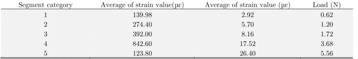
Figure 5(b) shows the strain signal segments that were extracted after the editing process by means of the Wavelet Transform analysis. Through this editing process, it could be seen that low amplitude segments had been eliminated because these segments concerned did not contribute to fatigue damage. As many as 21 segments can be retained after the editing process. The segments concerned were then classified in five categories based on the amplitude values, which were then averaged. The value of the strain signals that were retained based on these categories was then used to calculate the stress value by using the Ramberg-Osgood approach. Then, the load was obtained based on the relevant stress value. The overall results are shown in Table 3. Based on the results, the CAL load that was used was very small because the load that was applied to the coil spring during the SAE test was small compared to the strength of the material.
Segment category Average of strain value(µɛ) Average of strain value (µɛ) Load (N)
1 139.98 2.92 0.62
2 274.40 5.70 1.20
3 392.00 8.16 1.72
4 842.60 17.52 3.68
5 123.80 26.40 5.56
Table 3: Strain, stress and load values based on extracted segments.
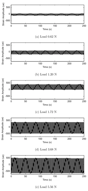
Figure 6 shows the strain signal that was obtained from the laboratory experiments using the CAL loading based on the SAE strain signal. According to the results that were obtained, the range of the strain signal increased with an increase in the applied load. The amplitude of this strain signal contributed to fatigue damage for the coil spring based on the editing process using the Wavelet Transform analysis. To predict the fatigue life for all the stages of this strain signal amplitude, an
0 20 40 60 80 100 120
-1,000-800 -600 -400 -2000 200 400 600 800 1,000
Time (s)
St
ra
in
A
mpl
itude (
ue)
0 20 40 60 80 100 120
-1,000-800 -600 -400 -2000 200 400 600 800 1,000
St
ra
in
A
m
pli
tu
de
(u
e)
analysis was conducted based on the strain-life approach. Since the strain signal obtained had a zero mean, the Coffin Manson model was used.
(a) Load 0.62 N
(b) Load 1.20 N
(c) Load 1.72 N
(d) Load 3.68 N
(e) Load 5.56 N
Figure 6: Strain signals that were collected during the laboratory experiments.
0 50 100 150 200 250
-500 0 500 Time (s) St ra in A m plit ud e (u e)
0 50 100 150 200 250
-500 0 500 Time (s) St ra in Am plit ud e (u e)
0 50 100 150 200 250
-500 0 500 Time (s) St ra in Am plit ud e (u e)
0 50 100 150 200 250
-500 0 500 Time (s) St ra in A m pl itud e (u e)
0 50 100 150 200 250
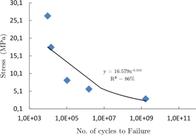
According to the guidelines in the fatigue life analysis, the S-N curve for the CAL loading was plotted in a semi-log or log-log scale containing experimental data. Figure 7 gives the semi-log plot for stress based on the SAE strain signal segment against the number of failure cycles for the SAE 5016 specimen. This S-N curve showed the general trend for the increase in fatigue life by a reduction in the stress amplitude, which is normally obtained from other types of steel. The S-N curve, which models the experimental data, is shown in Equation (7):
σ = 16.58 (Nf) -0.16 (7)
where σ is the stress amplitude and Nf is the number of failed cycles. The value of R2 for the S-N
curve was 86%. The regression based on the data from the plot of the curve was good. The long fatigue life showed that the specimen had a much higher strength
Figure 7: S-N curve based on stress values obtained from laboratory experiments under CAL loading.
In this study, 2-parameter Weibull distribution model was used to analyse the fatigue life based on the strain signal. The advantage of using this distribution is that it can be explained by a simple function, and it is often used to evaluate the fatigue life of the material based on a simple calculation (Godez et. al, 2013). Table 3 shows the results that were obtained from the Weibull analysis.
Based on the results obtained in Table 4, the shape parameter, β for the data obtained from the laboratory experiment was less than two. This indicates that the data obtained had a decreased failure rate. The scale parameter, θ of 2.56 x 10⁷ obtained showed that when the rotating load achieved the relevant cycles, the structure of the specimen changed and resulted in a high probability for failure. The reliable life was also taken into account in the probability analysis because it gave the life cycle that was involved when the operation or test was being conducted. The specimen would remain in a safe condition during the operation in the reliable life cycle without the involvement of any change in the circumstances that would cause the specimen to fail. The Mean time to Failure (MTTF) is the number of operational cycles that are required before failure is experienced. With reference to the
number of MTTF cycles, i.e. 2.83 x 10¹², when the cycles reach the value concerned, there is a
possibility that the specimen will fail or fracture.
y = 16.579x-0.164
R² = 86%
, 5, , 5, , 5, ,
, E+ , E+ 5 , E+ 7 , E+ 9 , E+
Stress
(M
P
a)
Parameters value
Shape parameter, β 0.12
Scale parameter,θ 2.56 x 10⁷
Reliable life, cycle 9360
Mean time to failure MTTF, cycle 2.83 x 10¹²
Table 4: Results of Weibull Distribution analysis.
Figure 8 shows the plot for the probability density function (PDF) that refers to the interpretation of the mathematical functions for time to attain failure based on the number of cycles. The PDF distribution shows that the plot was more inclined towards the right and decreased when it got closer to the value of the stress that was applied to the specimen. This distribution was because the value of the shape parameter, β that was obtained was less than two and had a reduced failure rate. The cumulative density function (CDF) is a plot of the value of every observation of the percentage in the sample that is less or equal to the relevant value (Sivapragash et al., 2008). In this study, the CDF was used to determine the percentage of specimens that failed during the experiment based on the number of cycles. Figure 9 shows the CDF plot for the experiment that was conducted. According to the plot that was obtained, more than 80% of the failures will occur at 1.7 x 10¹¹ cycles if the 2.92 MPA stress was applied.
Figure 8: Plot of probability distribution function (PDF).
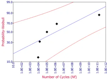
The Weibull cumulative probability plot at a confidence level of 95% for the number of failure cycles for the laboratory experiment is shown in Figure 10. The number of failure cycles at a certain percentage of probability subject to the applied load can be known through this plot. For example, 50% of the probability of failure in the specimen occurred at 1.0 x 10⁶ cycles and more than 70% will occur at more than 1.0 x 10¹¹ cycles. This value was an indicator that helped to predict the fatigue life in the experiments that were conducted. Therefore, the life cycles that lead to failure can be roughly determined by using the Weibull distribution probability method.
Figure 10: Plot of probability of failure against number of cycles.
5 CONCLUSION
The value of the damage retained during the editing of the strain signal can be used to design a new strain signal for a CAL load that is equivalent to the actual condition derived from the VAL load. The laboratory experiments that were carried out based on the stress value obtained from the con-version of the strain using the Ramberg-Osgood equation showed that the higher the stress, the lower the value of the life cycle. This was supported by a probability analysis using the Weibull distribution method that led to a statistical evaluation. The PDF, CDF and probability of failure plots showed
that more than 70% of failures occurred when the number of cycles approached 1.0 x 10¹¹. Apart
from the conventional analysis, statistical procedures can also be carried out for the verification pro-cess. Therefore, the Weibull distribution analysis can be used as an alternative for predicting the percentage probability of failure.
Acknowledgment
References
Chang C. C. and Chen L.W., (2005). Detection of the location and size of cracks in the multiple cracked beam by spatial wavelet based approach, Mechanical System and Signal Processing 19(1): 139-155.
Colin, R.G. and Peter, R.L. (2009). In-service fatigue failure of engineered products and structures: Case study review, Engineering Failure Analysis 16 (6): 1775-1793.
Glodez, S., Sori M. and Kramberger, J. (2013). Prediction of Micro-Crack Initiation in High Strength Steels Using Weibull Distribution, Engineering Fracture Mechanics 108: 263-274.
Gupta, S., Ray, A. and Keller, E. (2006). Symbolic time series analysis of ultrasonic for fatigue damage monitoring in polycrystalline alloys, Measurement Science and Technology 1: 1963-1973.
Lee, Y.-L., Pan, J., Hathway, R.B. and Barkey, M.E. (2005), Fatigue Testing and Analysis (Theory and Practice), Butterworh-Heinemann, Oxford.
Lee D. C. and Han, C. S. (2009). CAE (computer aid engineering) driven durability model verification for the auto-motive structure development, Finite Element in Analysis and Design 45 (5): 324-332.
Mansor, N. I. I., Abdullah, S. and Ariffin, A. K. (2017). Descerning the fatigue crack growth behaviour of API X65 steels under sequence loading, Latin American Journal of Solids and Structures 14(02): 202-216.
Piotrkowski, P., Castro, E., and Gallego, A., (2009). Wavelet power, entropy and bispectrum applied to AE signals for damage identification and evaluation of corroded galvanized steel, Mechanical System and Signal Processing 23 (2): 432-445.
Post, N. L., Case, S. W. and Lesko, J. J. (2008). Modelling the variable amplitude fatigue of composite materials, International. Journal of Fatigue, 30: 2064–86.
Rahman, M. M., Kadirgama, K., Noor, M. M., Rejab, M. R. M. and Kesulai, S. A. (2009). Fatigue life prediction of lower suspension arm using strain life approach, European Journal of Scientific Research, 30(3): 437-450.
Sifuzzaman, M., Islam, M. R, and Ali, M. Z., (2009). Application of wavelet transform and its advantages compared to fourier transform, Journal of Physics and Science 13: 121-134.
Sivapragash, M., Lakshminarayanan, P. R., Karthikeyen, R., Raghukandan, K. and Hanumantha M. (2008). Fatigue life prediction of ZE41A magnesium alloy using Weibull distribution, Materials & Design, 29: 1549–53.
Stephens, R. I., Dindinger, P. M. and Gunger, J. E. (1997). Fatigue damage editing for accelerated durability testing using strain range and SWT parameter criteria. International Journal of Fatigue 19(8-9): 599 – 606.
Tsapi Tchoupau, K. M., Soh Fotsing, B. D. (2015). Fatigue equavailent stress state approach validation in non-conservative criteria: a comparative study, Latin American Journal of Solids and Structures 12(13): 2506-2519 Wang, W. J. and McFadden, P. D. (1995). Application of orthogonal wavelets to early gear damage detection. Me-chanical Systems and Signal Processing, 9 (5): 497-507.
Wei, L. W., de los Rios, E. R. and James, M. N. (2002). Experimental study and modelling of short fatigue crack growth in aluminium alloy A17010-T7451 under random loading, International Journal Fatigue 24: 963–75.