Abstract
In this paper, a new higher-order layerwise finite element model, de-veloped earlier by the present authors for the static analysis of lam-inated composite and sandwich plates, is extended to study the free vibration behavior of multilayer sandwich plates. In the present layerwise model, a first-order displacement field is assumed for the face sheets, whereas a higher-order displacement field is assumed for the core. Thanks for enforcing the continuity of the interlaminar dis-placement, the number of variables is independent of the number of layers. In order to reduce the computation effort, a simply four-noded C0 continuous isoparametric element is developed based on the
pro-posed model. In order to study the free vibration, a consistent mass matrix is adopted in the present formulation. Several examples of laminated composite and sandwich plate with different material com-binations, aspect ratios, boundary conditions, number of layers, ge-ometry and ply orientations are considered for the analysis. The per-formance and reliability of the proposed formulation are demon-strated by comparing the author’s results with those obtained using the three-dimensional elasticity theory, analytical solutions and other advanced finite element models. From the obtained results, it can be concluded that the proposed finite element model is simple and ac-curate in solving the free vibration problems of laminated composite and sandwich plates.
Keywords
Layerwise, Finite element, Laminated composite, Sandwich plates, Static, Free vibration.
On the Free Vibration Analysis of Laminated Composite
and Sandwich Plates: A Layerwise Finite Element Formulation
1 INTRODUCTION
Due to their low weight, high stiffness and high strength properties, the composites sandwich
struc-tures are widely used in various industrial areas e.g. civil constructions, marine industry, automobile
Mohamed-Ouejdi Belarbi
a, *Abdelouahab Tati
aHoudayfa Ounis
aAbdelhak Khechai
ba Laboratoire de Génie Energétique et
Matériaux, LGEM. Université de Biskra, B.P. 145, R.P. 07000, Biskra, Algeria. E-mail: [email protected], [email protected],
b Laboratoire de Recherche en Génie
Civil, LRGC. Université de Biskra, B.P. 145, R.P. 07000, Biskra, Algeria. E-mail: [email protected]
* Corresponding author
http://dx.doi.org/10.1590/1679-78253222
and aerospace applications. A sandwich is a three layered construction, where a low weight thick core
layer (e.g., rigid polyurethane foam) of adequate transverse shear rigidity, is sandwiched between two
thin laminated composite face layers of higher rigidity (Pal and Niyogi 2009). Despite the many
advantages of sandwich structures, their behavior becomes very complex due to the large variation
of rigidity and material properties between the core and the face sheets. Therefore, the accuracy of
the results for sandwich structures largely depends on the computational model adopted (Pandey and
Pradyumna 2015).
In the literature, several two-dimensional theories and approaches have been used to study the
behavior of composite sandwich structures. Starting by the simple classical laminated plate theory
(CLPT), based on the Kirchhoff’s assumptions, which does not includes the effect of the transverse
shear deformation, the first-order shear deformation theory (FSDT), where the effect of the transverse
shear deformation is considered (Reissner 1975, Whitney and Pagano 1970, Mindlin 1951, Yang et al.
1966), but this theory gives a state of constant shear stresses through the plate thickness, and the
higher-order shear deformation theories (HSDT) where a better representation of transverse shear effect
can be obtained (Lo et al. 1977, Manjunatha and Kant 1993, Reddy 1984, Lee and Kim 2013). Regarding
the approaches used to model the behavior of composite structures, we distinguish the equivalent single
layers (ESL) approach where all the laminate layers are referred to the same degrees-of-freedom (DOFs).
The main advantages of ESL models are their inherent simplicity and their low computational cost, due
to the small number of dependent variables. However, ESL approach fails to capture precisely the local
behavior of sandwich structures. This drawback in ESL was circumvented by the Zig-Zag (ZZ) and
layerwise (LW) approaches in which the variables are linked to specific layers (Belarbi and Tati 2015,
Belarbi et al. 2016,
Ć
etkovi
ć
and Vuksanovi
ć
2009, Chakrabarti and Sheikh 2005, Kapuria and Nath
2013, Khalili et al. 2014, Khandelwal et al. 2013, Marjanovi
ć
and Vuksanovi
ć
2014, Maturi et al. 2014,
Sahoo and Singh 2014, Singh et al. 2011, Thai et al. 2016). For more details, the reader may refer to
(Carrera 2002, Ha 1990, Khandan et al. 2012, Sayyad and Ghugal 2015).
In the last decades, the finite element method (FEM) has become established as a powerful
method and as the most widely used method to analyze the complex behavior of composite sandwich
structures (e.g., bending, vibration, buckling). This is due to the limitations in the analytical methods
which are applicable only for certain geometry and boundary conditions (Kant and Swaminathan
2001, Mantari and Ore 2015, Maturi et al. 2014, Noor 1973, Plagianakos and Papadopoulos 2015,
Srinivas and Rao 1970). Khatua and Cheung (1973) were one of the first to use the FEM in the
analysis of this type of structures. They developed two triangular and rectangular elements to study
the bending and free vibration of sandwich plates.
Chalak et al. (2013) developed a nine node finite element by taking out the nodal field variables
in such a manner to overcome the problem of continuity requirement of the derivatives of transverse
displacements for the free vibration analysis of laminated sandwich plate. An efficient nine-noded
quadratic element with 99 DOFs is developed by Khandelwal et al. (2013) for accurately predicting
natural frequencies of soft core sandwich plate. The formulation of this element is based on combined
theory, HZZT and least square error (LSE) method. Therefore, the zig-zag plate theory presents good
performance but it has a problem in its finite element implementation as it requires C
1continuity of
transverse displacement at the nodes which involves finite element implantation difficulties. Also, it
requires high-order derivatives for displacement when obtaining transverse shear stresses from
equi-librium equations (Pandey and Pradyumna 2015).
Recently, various authors have adopted the layerwise approach to assume separate displacement
field expansions within each material layer. Lee and Fan (1996) described a new layerwise model
using the FSDT for the face sheets whereas the displacement field at the core is expressed in terms
of the two face sheets displacements. They used a nine-nodded isoparametric finite element for
bend-ing and free vibration of sandwich plates. On the other hand, a new three-dimensional (3D) layerwise
finite element model with 240 DOFs has been developed by Nabarrete et al. (2003) for dynamic
analyses of sandwich plates with laminated face sheets. They used the FSDT for the face sheets,
whereas for the core a cubic and quadratic function for the in-plane and transverse, displacements,
was adopted. In the same year, Desai et al. (2003) developed an eighteen-node layerwise mixed brick
element with 108 DOFs for the free vibration analysis of multi-layered thick composite plates. Later,
an eight nodes quadrilateral element having 136 DOFs was developed by Araújo et al. (2010) for the
analysis of sandwich laminated plates with a viscoelastic core and laminated anisotropic face layers.
The construction of this element is based on layerwise approach where the HSDT is used to model
the core layer and the face sheets are modeled according to a FSDT. Elmalich and Rabinovitch (2012)
have undertaken an analysis on the dynamics of sandwich plates, using a C0 four-node rectangular
element. The formulation of this element is based on the use of a new layerwise model, where the
FSDT is used for the face sheets and the HSDT is used for the core. In 2015, Pandey and Pradyumna
(2015) presented a new higher-order layerwise plate formulation for static and free vibration analyses
of laminated composite plates. A high-order displacement field is used for the middle layer and a
first-order displacement field for top and bottom layers. The authors used an eight-noded isoparametric
element containing 104 DOFs to model the plate. The performance of these layerwise models is good
but it requires high computational effort as the number of variables dramatically increases with the
number of layers.
model are compared favorably with those obtained via analytical solution and numerical results
ob-tained by other models. The results obob-tained from this investigation will be useful for a more
under-standing of the bending and free vibration behavior of sandwich laminates plates.
2 MATHEMATICAL
MODEL
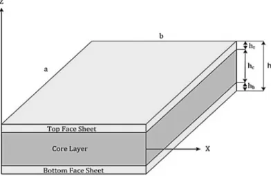
Sandwich plate is a structure composed of three principal layers as shown in Figure.1, two face sheets
(top-bottom) of thicknesses (
h
t), (
h
b) respectively, and a central layer named core of thickness (
h
c)
which is thicker than the previous ones. Total thickness (
h
) of the plate is the sum of these thicknesses.
The plane (
x, y
) coordinate system coincides with mid-plane plate.
Figure 1: Geometry and notations of a sandwich plate.
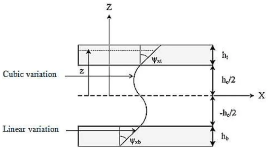
2.1 Displacement Field
In the present model, the core layer is modeled using the HSDT. Hence, the displacement field is
written as a third-order Taylor series expansion of the in-plane displacements in the thickness
coor-dinate, and as a constant one for the transverse displacement:
2 3
0
2 3
0
0
c c c
c x x x
c c c
c y y y
c
u
u
Z
Z
Z
v
v
Z
Z
Z
w
w
(1)
where
u
0,
v
0and
w
0are respectively, in-plane and transverse displacement components at the
mid-plane of the sandwich plate.
c,
cx y
represent normal rotations about the x and y axis respectively.
The parameters
cx
,
cy
,
c x
and
c y
are higher order terms.
Figure 2: Representation of layerwise kinematics and coordinate system.
a) Top face sheet
0
2
2
2
2
t
c c
t c x
t
c c
t c y
t
h
h
u
u
Z
h
h
v
v
Z
w
w
(2)
where
t x
and
ty
are the rotations of the top face-sheet cross section about the y and x axis,
respec-tively, and the displacement of the core for (z=
h
c/2) is given by:
2 3
0
2 3
0
2
2
4
8
2
2
4
8
c c c
c c c c
c x x x
c c c
c c c c
c y y y
h
h
h
h
u
u
h
h
h
h
v
v
(3)
The substitution of Eq. (3) in Eq. (2) led finally to the following expressions:
2 3
0
2 3
0
0
2
4
8
2
2
4
8
2
c c c t
c c c c
t x x x x
c c c t
c c c c
t y y y y
t
h
h
h
h
u
u
Z
h
h
h
h
v
v
Z
w
w
(4)
b) Bottom face sheet
0
2
2
2
2
b
c c
b c x
b
c c
b c y
b
h
h
u
u
Z
h
h
v
v
Z
w
w
(5)
where
b x
and
b y
are the rotations of the bottom face-sheet cross section about the y and x axis
respectively, and the displacement of the core for (z=-
h
c/2) is given by:
2 3
0
2 3
0
2
2
4
8
2
2
4
8
c c c
c c c c
c x x x
c c c
c c c c
c y y y
h
h
h
h
u
u
h
h
h
h
v
v
(6)
Substituting equation (6) into equation (5), leads to the following expression:
2 3
0
2 3
0
0
2
4
8
2
2
4
8
2
c c c b
c c c c
b x x x x
c c c b
c c c c
b y y y y
b
h
h
h
h
u
u
Z
h
h
h
h
v
v
Z
w
w
(7)
2.2 Strain–Displacement Relations
The strain-displacement relations derived from the displacement model of Eqs. (1), (4) and (7) are
given as follows:
For the core layer,
2 3 0 2 3 0 2 3 0 0 2
0
2
3
c c c
c x x x
xx
c c c
y y y
c yy
c c c
c c c
y y y
c x x x
xy
c c c c
yz y y y
c c
xz x
u
Z
Z
Z
x
x
x
x
v
Z
Z
Z
y
y
y
y
u
v
Z
Z
Z
y
x
y
x
y
x
y
x
w
Z
Z
y
02
c 23
cx x
w
Z
Z
x
(8)
2 3 2 3 0 0 0 0 ( )
2 4 8 2
( )
2 4 8 2
c c c t
t c x c x c x c x
c c c t
y y y y
t c c c c
t t c
t xx t yy t xy
u h h h h
x x x x x
v h h h h
y y y y y
u v u v h
y x y x
u
Z
x
v
Z
x
2 0 0 3 2 4 ( ) 8 2c c c c y y
x c x
c t
c t
y y
c x c
t y t x x t yz t xz h
y x y x
h w y w x h
y x
Z
y x
(9)
For the bottom face sheet,
2 3 0 2 3 0 0 0 ( )
2 4 8 2
( )
2 4 8 2
c c c b
b c x c x c x c x
c c c b
y y y y
b c c c c
b b c
b xx b yy b xy
u u h h h h
x x x x x x
v v h h h h
y y y y y y
u v u v h
y x y x
Z
Z
2 3 2 4 ( ) 8 2c c c c y y
x c x
c b
c b
y y
c x c x
h
y x y x
h h
y x
Z
y x
0 0 b y b x b yz b xz w y w x
(10)
2.3 Constitutive Relationships
In this work, the two face sheets (top and bottom) are considered as laminated composite. Hence, the
stress-strain relations for
thk
layer in the global coordinate system are expressed as:
11 12 16
21 22 26
44 45
54 55
61 62 66
0 0 0 0
,
0 0 0
0 0 0
0 0
f f xx xx f f yy yy f f yz yz f f xz xz f f xy xy k
k Q Q Q k
Q Q Q
f top bottom
Q Q
Q Q
Q Q Q
The core is considered as an orthotropic composite material and its loads resultants are obtained
by integration of the stresses through the thickness direction of laminated plate.
2 2 3 2 2 2 21, , ,
1, , c c c c h
x x x x x
y y y y y
h
xy
xy xy xy xy
h
x x x xz
y y y h yz
N M N M
N M N M Z Z Z d
N M N M
V S R
Z Z d
V S R
z
z
(12)
where
N M,denote membrane
effort, bending moment, respectively, and
N,
M
denote higher order
membrane and moment resultants, respectively.
V
is the shear resultant;
S
and
R
are the higher order
shear resultant.
It is informative to relate the loads resultants of the core defined in Eq. (12) to the total strains
in Eq. (8). From Eqs. (8) and (12), we obtain:
0 1 2 3N A B D E
M B D E F
D E F G
N
E F G H
M
(13a)
0 1 2s s s
s
s s s
s
s s s
s
A B D
V
S B D E
R D E F
(13b)
where
A , Bij ij, etc. are the elements of the reduced stiffness matrices of the core, defined by:
2
2 3 4 5 6
2
2
2 3 4
2
, , , , , , 1, , , , , , ( , 1, 2,6)
, , , , 1, , , , ( , 4,5)
c c c c ij ij h
ij ij ij ij ij ij ij h
h
s s s s s
ij ij ij ij ij h
c
c
A B D E F G H Q Z Z Z Z Z Z d i j
A B D E F Q Z Z Z Z d i j
z
z
(14)
According to the FSDT, the constitutive equations for the two face sheets are given by:
0 0 0 0
f f f f
m
f f f f
f
f f f
c c
N A B
M D T A
B
(15)
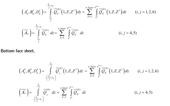
a. Top face sheet,
1
1 2
2 2
2
2
2
( ) ( )
1
( ) ( )
1
, , 1, , 1, , ( , 1, 2,6)
( , 4,5)
c t
c
c t
c
k
k
k
k h
h
h
h h
h h
h t
ij
h h
n layer
k k
t t t
ij ij
ij ij ij
k
n layer
k k
ij ij
k
A B D Q Z Z dz Q Z Z dz i j
Q dz Q dz i j
A
(16)
b. Bottom face sheet,
1
1 2
2 2
2
2
2
( ) ( )
1
( ) ( )
1
, , 1, , 1, , ( , 1, 2,6)
c
c b
c
c b
k
ij
k
k
ij
k h
h
h h
h
h
h b
ij
h h h
n layer
k k
b b b
ij ij ij ij
k
n layer
k k
ij k
A B D Q Z Z dz Q Z Z dz i j
Q dz Q dz
A
( ,i j4,5)(17)
3 FINITE ELEMENT FORMULATION
In the present study, a four-node C
0continuous quadrilateral element, named QSFT52 (Quadrilateral
Sandwich First Third with 52-DOFs), with thirteen DOFs per node
0 0 0
T
c c c c c c t t b b
x y x y x y x y x y
u v w
has been developed. Each node contains: two
rota-tional DOF for each face sheet, six rotarota-tional DOF for the core, while the three translations DOF are
common for sandwich layers (Figure.3).
The displacements vectors at any point of coordinates (x, y) of the plate are given by:
1
,
, n i i
i
x y
x y N
(18)
where
iis the nodal unknown vector corresponding to node i (
i
= 1, 2 3 4),
N
iis the shape function
associated with the node
i
.
The generalized strain vector for three layers can be expressed in terms of nodal displacements
vector as follows:
( ) ( )
i
k k
i
B
(19)
where the matrices
( )k iB
relate the strains to nodal displacements.
4 GOVERNING DIFFERENTIAL EQUATION
In this work, Hamilton’s principle is applied in order to formulate governing free vibration problem,
which is given as:
2
1
0
tt
T
U dt
(20)
where
t
is the time,
T
is the kinetic energy of the system and
U
is the potential energy of the system.
The first variation of kinetic energy of the three layers sandwich plate can be expressed as:
t
c
b V
V
V
t t t t t t t t
c c c c c c c c
b b b b b b b b
T
u u
v v
w w dV
u u
v v
w w dV
u u
v v
w w dV
(21)
where
u
i,
v
iand
w
iare the displacement in
x,y
and
z
directions, respectively, of the three-layered
sandwich (
i = t, c, b
),
iand
V
iare the density of the material and volume, of each component,
respectively, and (
..) is a second derivative with respect to time.
The first variation of the potential energy of the sandwich plate is the summation of contribution
from the two face sheets and from the core as:
2
2
2
2
c
c c
c t
c
t h
c c c c c c c c c c
xx xx yy yy xy xy xz xz yz yz
A h
h h
t t t t t t t t t t
xx xx yy yy xy xy xz xz yz yz
A h
c
t
U
dV
dV
2 2c c b b h
b b b b b b b b b b
xx xx yy yy xy xy xz xz yz yz
A h h b
dV
In the present analysis, the work done by external forces and the damping are neglected. Hence,
Eq. (20) leads to the following dynamic equilibrium equation of a system.
M
e
K
e
0
(23)
where
M
eand
K
edenote the total element mass matrix and the total element stiffness matrix
respectively, which are computed using the Gauss numerical integration. The total element stiffness
matrix is the summation of contribution from the two face sheets and from the core as:
t c be e e e
K
K
K
K
(24)
where the element stiffness matrix of the core
c eK
are given by,
1 0 1 1
1 2 1 3 2 0
0 0 0 1 0 2
0 3 T T
T T T
c T T T
T e
B B B B D B
B E B B F B B D B
B
A B
B
B
B
B
D
B
B
E
B
K
2 1 2 2 2 3
3 0 3 1 3 2
0 0 0
3 3
s s s
T T T
T T T
T T
T
s
B E B B F B B L B
B E B B F B B L B
B H B B A B B B
10 2 1 0 1 1
1 2 2 0 2 1
s
s s s s s s
s s s s s s
s
T T T
s s s
T T T
s s s
B
B D B B B B B D B
B E B B D B B E B
2 2
s s
T s
B F B dA
(25)
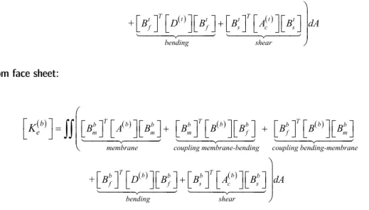
For the two face sheets, the element stiffness matrix can be written as:
a. Top face sheet:
t T t t t T t t t T t t
m m m f f m
t e
membrane coupling membrane-bending coupling bending-membrane
B A B B B B B B B
K
T t T t
t t t t
f f s c s
bending shear
+ B D B B A B dA
b. Bottom face sheet:
b T b b b T b b b T b b
m m m f f m
b f b
e
membrane coupling membrane-bending coupling bending-membrane
B A B B B B B B B
+ B
K
T b b b T b b
f s c s
bending shear
D B B A B dA
(27)
The total element mass matrix, for the three-layer sandwich plate, can be written as
T ( )t
T ( )c
+
T ( )b
e
M
N
m
N
N
m
N
N
m
N
dA
(28)
where
( )tm
,
m
( )c
and
m
( )b
are the consistent mass matrices of the top face sheet, core and the
bottom face sheet, respectively, containing inertia terms. Now, after evaluating the stiffness and mass
matrices for all elements, the governing equations for free vibration analysis can be stated in the form
of generalized eigenvalue problem.
2
0
K
M
(29)
where,
denote the natural frequency,
Kis he global stiffness matrix,
M
is the global mass
matrix,
are the vectors de
fi
ning the mode shapes.
5 NUMERICAL RESULTS AND DISCUSSIONS
In this section, several examples on the free vibration analysis of laminated composite and sandwich
plates will be analyzed to demonstrate the performance and the versatility of the developed finite
element model. The MATLAB programming language is used to solve the eigenvalue problem. The
obtained numerical results are compared with the analytical solutions and others finite elements
numerical results found in the literature.
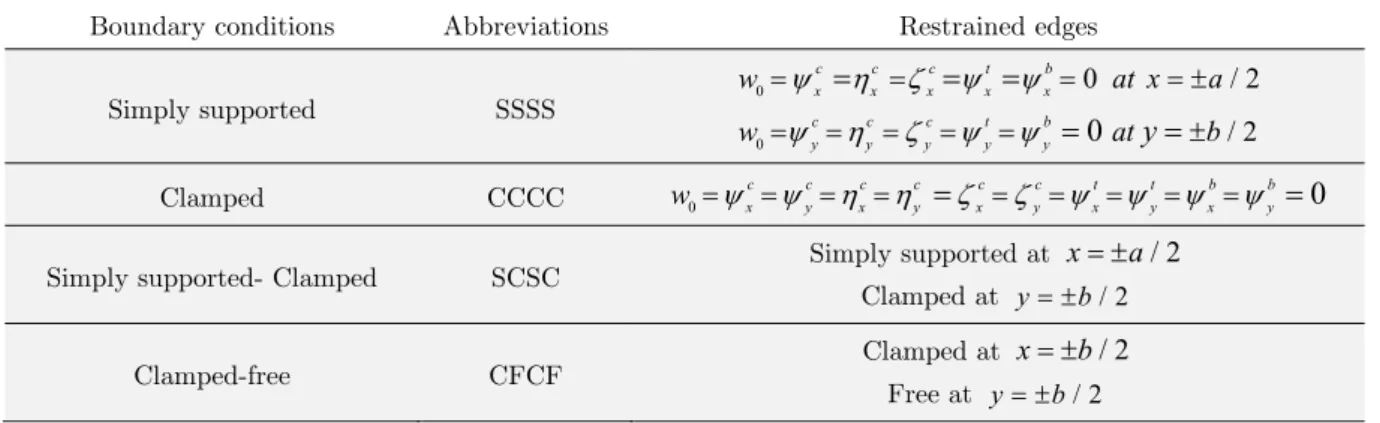
Boundary conditions Abbreviations Restrained edges
Simply supported SSSS 0
0
0 / 2
0
/ 2c c c t b
x x x x x
c c c t b
y y y y y
w at x a
w at
y
b
Clamped CCCC 0
0
c c c c c c t t b b
x y x y x y x y x y
w
Simply supported- Clamped SCSC Simply supported at x a/ 2
Clamped at y b/ 2
Clamped-free CFCF Clamped at x b/ 2
Free at y b/ 2
Table 1: Boundary conditions used in this study.
Elastic
properties Unit MM1 MM2 MM3 MM4 MM5 MM6 MM7 MM8
E
11 GPa 24.51 0.1036 276.0 0.5776 40Open
131.0 0.00690E
22 GPa 7.77 0.1036 6.9 0.5776E
22E
22 10.34 0.00690G
12 GPa 3.34 0.05 6.9 0.1079 0.6E
220.6
E
22 6.9 0.00344G
13 GPa 3.34 0.05 6.9 0.1079 0.5E
220.6
E
22 6.2 0.00344G
23 GPa 1.34 0.05 6.9 0.2221 0.5E
220.5
E
22 6.9 0.00345-
0.078 0.32 0.25 0.0025 0.250.25
0.22 10-5Kg/m3 1800 130 681.8 1000 1 1 1627 97
Table 2: Material models (MM) considered for different laminated and sandwich plate.
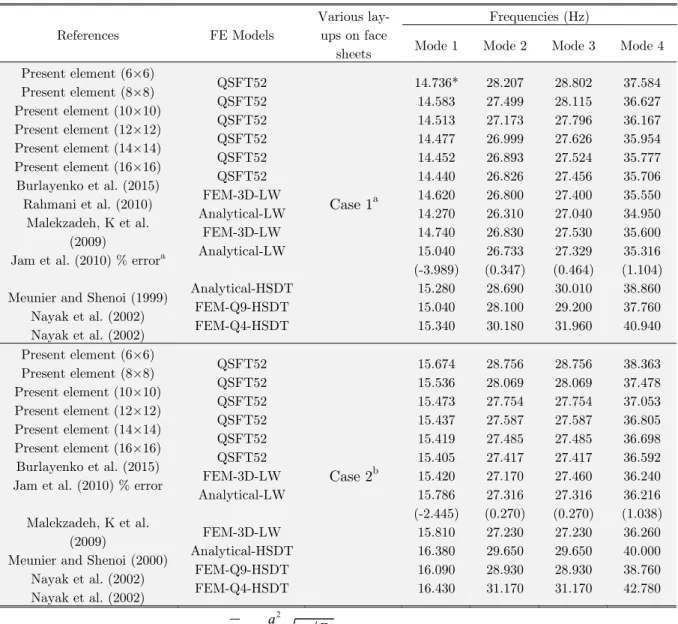
5.1 Convergence Study
In the first example, the convergence of the developed quadrilateral element is studied for a seven-
layer simply supported square sandwich plate. Two sandwich plates with various lay-ups on face
sheets [0/90/0/core/0/90/0] and [45/-45/45/core/-45/45/-45] are considered. The core is made of
HEREX-C70.130 PVC foam (MM1) and the face sheets are made of glass polyester resin (MM2). The
geometrical properties of the plate are (
a/h
= 10, a/b = 1,
hc
/
h
= 0.88) where h is the total thickness
of the plate. The convergence of the non-dimensional results of natural frequencies, for the
fi
rst four
modes, is shown in Table 3 with different mesh sizes (6×6, 8×8, 10×10, 12×12, 14×14 and 16×16).
The comparison was made with the analytical solutions based on LW approach (Jam et al. 2010,
Rahmani et al. 2010), the 3D-finite element models also based on LW approach (FEM-3D-LW)
(Ma-lekzadeh and Sayyidmousavi 2009, Burlayenko et al. 2015), the FEM-Q9 and Q4 solution based on
HSDT (Nayak et al. 2002) and other analytical solution based on HSDT (Meunier and Shenoi 1999).
The results of the comparison show the performances and convergence of the present formulation.
12
References FE Models Various
lay-ups on face sheets
Frequencies (Hz)
Mode 1 Mode 2 Mode 3 Mode 4
Present element (6×6) Present element (8×8) Present element (10×10) Present element (12×12) Present element (14×14) Present element (16×16) Burlayenko et al. (2015) Rahmani et al. (2010)
Malekzadeh, K et al. (2009)
Jam et al. (2010) % errora
Meunier and Shenoi (1999) Nayak et al. (2002) Nayak et al. (2002)
QSFT52 QSFT52 QSFT52 QSFT52 QSFT52 QSFT52 FEM-3D-LW Analytical-LW FEM-3D-LW Analytical-LW Analytical-HSDT FEM-Q9-HSDT FEM-Q4-HSDT
Case 1
a14.736* 14.583 14.513 14.477 14.452 14.440 14.620 14.270 14.740 15.040 (-3.989) 15.280 15.040 15.340 28.207 27.499 27.173 26.999 26.893 26.826 26.800 26.310 26.830 26.733 (0.347) 28.690 28.100 30.180 28.802 28.115 27.796 27.626 27.524 27.456 27.400 27.040 27.530 27.329 (0.464) 30.010 29.200 31.960 37.584 36.627 36.167 35.954 35.777 35.706 35.550 34.950 35.600 35.316 (1.104) 38.860 37.760 40.940
Present element (6×6) Present element (8×8) Present element (10×10) Present element (12×12) Present element (14×14) Present element (16×16) Burlayenko et al. (2015) Jam et al. (2010) % error
Malekzadeh, K et al. (2009)
Meunier and Shenoi (2000) Nayak et al. (2002) Nayak et al. (2002)
QSFT52 QSFT52 QSFT52 QSFT52 QSFT52 QSFT52 FEM-3D-LW Analytical-LW FEM-3D-LW Analytical-HSDT FEM-Q9-HSDT FEM-Q4-HSDT
Case 2
b15.674 15.536 15.473 15.437 15.419 15.405 15.420 15.786 (-2.445) 15.810 16.380 16.090 16.430 28.756 28.069 27.754 27.587 27.485 27.417 27.170 27.316 (0.270) 27.230 29.650 28.930 31.170 28.756 28.069 27.754 27.587 27.485 27.417 27.460 27.316 (0.270) 27.230 29.650 28.930 31.170 38.363 37.478 37.053 36.805 36.698 36.592 36.240 36.216 (1.038) 36.260 40.000 38.760 42.780
* The natural frequencies are expressed as:
a Percentage error = [(Present result - Analytical result) / Analytical result] × 100
b Various lay-ups on face sheets : Case 1: [0/90/0/core/0/90/0] and Case 2 : [45/-45/45/core/-45/45/-45].
Table 3: Non-dimensional natural frequencies for a square multi-layered sandwich plate with various lay-ups on face sheets.
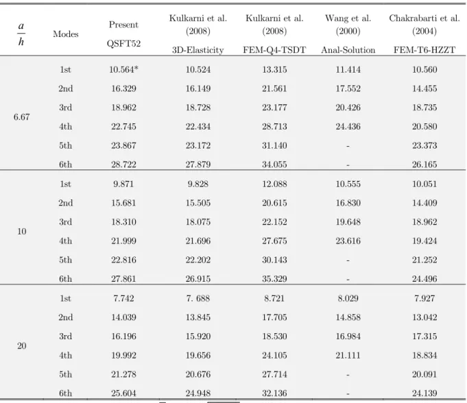
5.2 Square Sandwich Plate (0/90/C/90/0) Having Two-Ply Laminated Stiff Sheets at the Faces
In this problem, a simply supported square sandwich plate having two laminated stiff layers is
inves-tigated. The thickness of each laminate layer is 0.05h, whereas the thickness of the core is 0.8h. The
mechanical properties MM3 and MM4 of table 2 are adopted, respectively, for laminated face sheets
and core. The non-dimensional natural frequencies, for the
fi
rst six modes, are presented in table 4
using a mesh size of 12×12. In the present analysis, different thickness ratios (
a/h
= 6.67, 10 and 20)
are considered. The obtained results are compared with the 3D-elasticity solution given by Kulkarni
and Kapuria (2008), analytical results of Wang et al. (2000) using p-Ritz method and some existing
finite element results based on HZZT (Chakrabarti and Sheikh 2004, Kulkarni and Kapuria 2008). It
is clear, from the table 4, that the results of developed element are in excellent agreement with
numerical results found in the literature.
Modes Present
QSFT52
Kulkarni et al. (2008)
3D-Elasticity
Kulkarni et al. (2008)
FEM-Q4-TSDT
Wang et al. (2000)
Anal-Solution
Chakrabarti et al. (2004)
FEM-T6-HZZT
6.67
1st
2nd
3rd
4th
5th
6th
10.564*
16.329
18.962
22.745
23.867
28.722
10.524
16.149
18.728
22.434
23.172
27.879
13.315
21.561
23.177
28.713
31.140
34.055
11.414
17.552
20.426
24.436
-
-
10.560
14.455
18.735
20.580
23.373
26.165
10
1st
2nd
3rd
4th
5th
6th
9.871
15.681
18.310
21.999
22.816
27.861
9.828
15.505
18.075
21.696
22.202
26.915
12.088
20.615
22.152
27.675
30.143
35.329
10.555
16.830
19.648
23.616
-
-
10.051
14.409
18.962
19.424
21.252
24.496
20
1st
2nd
3rd
4th
5th
6th
7.742
14.039
16.196
19.992
21.278
25.604
7. 688
13.845
15.920
19.656
20.676
24.948
8.721
17.705
18.530
24.105
27.714
32.136
8.029
14.858
16.984
21.111
-
-
7.927
13.042
17.315
18.834
20.091
24.139 * The natural frequencies are expressed as:
Table 4: Non-dimensional fundamental frequencies with different modes for simply supported sandwich plate with laminated face sheets (0/90/C/90/0).
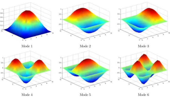
Moreover, the same plate is analyzed by considering two different boundary conditions, CCCC
and SCSC. The non-dimensional natural frequencies, for the
fi
rst six modes, are reported in table 5
for different thickness ratios (
a/h
= 5, 10 and 20). The first six mode shapes obtained for SSSS, CFCF
and CFFF square laminated sandwich plate with a/h =10 are shown in Figures 4, 5 and 6. It can be
observed that, in comparison with the FEM solution based on HZZT (Khandelwal et al. 2013, Chalak
et al. 2013, Kulkarni and Kapuria 2008, Chakrabarti and Sheikh 2004), the present element gives
more accurate results than the other models.
a
h
11
100 a c E f
Bound-ary condition Mode s Present QSFT52 Khandelwal et al. (2013) FEM-Q9-HZZT
Chalak et al. (2013)
FEM-Q9-HZZT
Kulkarni et al. (2008) FEM-Q4-HZZT Chakrabarti et al. (2004) FEM-T6-HZZT 5 SCSC 1st 2nd 3rd 4th 5th 6th 11.445 18.267 19.707 24.448 27.657 29.866 11.591 17.108 20.409 24.079 24.593 29.989 11.408 18.014 19.485 24.086 26.559 29.014 11.516 18.379 19.626 24.722 27.409 29.231 11.063 15.199 18.255 19.781 20.127 22.907 CCCC 1st 2nd 3rd 4th 5th 6th 12.200 18.733 21.120 25.614 27.959 29.866 12.121 18.453 20.706 25.058 26.849 30.908 12.138 18.469 20.764 25.138 26.860 31.050 12.440 19.106 21.442 26.691 28.043 32.257 11.864 15.672 19.477 20.057 21.167 23.628 10 SCSC 1st 2nd 3rd 4th 5th 6th 10.346 16.399 18.547 22.523 24.079 27.934 10.860 16.131 18.962 22.438 22.628 27.532 10.344 16.310 18.349 22.294 23.554 27.211 10.378 16.411 18.395 22.494 23.718 27.258 10.422 15.021 19.135 20.372 21.642 25.215 CCCC 1st 2nd 3rd 4th 5th 6th 11.318 16.967 19.332 23.187 24.428 27.934 11.349 16.900 19.214 23.003 23.925 28.502 11.356 16.909 19.236 23.041 23.935 28.539 11.468 17.135 19.494 23.659 24.253 28.918 11.524 15.691 19.946 20.783 22.356 25.812 20 SCSC 1st 2nd 3rd 4th 5th 6th 8.635 14.604 16.581 20.390 22.006 26.107 9.502 14.853 17.233 20.708 21.310 25.768 8.666 14.645 16.367 20.234 21.767 25.342 8.649 14.601 16.357 20.233 21.673 25.324 8.623 13.533 17.601 19.441 20.416 24.620 CCCC 1st 2nd 3rd 4th 5th 6th 10.253 15.530 17.605 21.217 22.568 26.107 10.330 15.598 17.644 21.246 22.354 26.636 10.336 15.609 17.659 21.278 22.368 26.683 10.332 15.600 17.674 21.404 22.323 26.893 10.536 14.709 18.708 20.182 21.369 25.406
Table 5: Non-dimensional fundamental frequencies for laminated sandwich plate (0/90/C/90/0) with different boundary conditions.
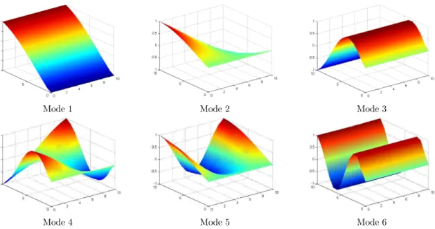
Mode 1 Mode 2 Mode 3
Mode 4 Mode 5 Mode 6
Figure 4: First six mode shapes of SSSS square laminated sandwich plate (0/90/C/90/0) with a/h =10.
Mode 1 Mode 2 Mode 3
Mode 4 Mode 5 Mode 6
Mode 1 Mode 2 Mode 3
Mode 4 Mode 5 Mode 6
Figure 6: First six mode shapes of CFFF square laminated sandwich plate (0/90/C/90/0) with a/h =10.