Lat. Am. j. solids struct. vol.14 número12

(1)

Abstract

There are typically three broad categories of structural optimization namely size, shape and topology. Over the past few decades various researchers have focused on developing techniques for optimizing structures by considering either one or a combination of these as-pects. In this paper the efficiency of these techniques are investigated in an effort to quantify the improvement of the result obtained by utilizing a more complex optimization routine. The percentage of the structural weight saved and computational effort required are used as measures to compare these techniques. The well-known genetic algorithm with elitism is used to perform these tests on various benchmark structures found in literature. Some of the results that are obtained include that a simultaneous approach produces, on av-erage, a 22 % better solution than a simple size optimization and a 12 % improvement when compared to a staged approach where the size, shape and topology of the structure is considered sequentially. From these results, it is concluded that a significant saving can be made by using a more complex optimization routine, such as a sim-ultaneous approach.

Keywords

Structural optimization, Genetic algorithms, Truss structures, Size, Shape and Topology optimization.

A Quantitative Comparison Between Size, Shape, Topology and

Simultaneous Optimization for Truss Structures

1 INTRODUCTION

Structural optimization has become an important part of structural design in recent years. With economical structures being the goal of almost all designs. Typically, the weight of a truss structure is used to measure efficiency as the assumption is made that the amount of material used is related to the resulting cost (Camp and Bichon, 2004).

Three aspects of a structure can be optimized including the size, shape and topology of the struc-ture. Each of these focus on different aspects of the strucstruc-ture. For example, size optimization refers

T.E. Müller a, * E. van der Klashorst b

a _{Department of Civil Engineering,}

Stellenbosch University, Stellenbosch, South Africa.

E-mail: [email protected] b _{Department of Civil Engineering,}

Stellenbosch University, Stellenbosch, South Africa. E-mail: [email protected]

* Corresponding author

http://dx.doi.org/10.1590/1679-78253900

(2)

to the physical size of the members within a structure, while shape refers to the geometric layout and topology to the internal member configuration of a structure (Mortazavi and Toğan, 2016).

What makes optimization problems difficult to solve is the size of the so-called search space. This relates to the number of variables present in the problem. With regard to structural problems, the number of variables and subsequently possible solutions can be vast and when constraints are in-cluded, such as a maximum stress or a deflection limit, the quest to arrive at a feasible solution becomes even more difficult. Another factor that influences the complexity of a structural problem is the mixture of different variables (Ahrari et al, 2015). These include discrete, continuous and boolean variables.

The process of solving an optimization problem typically involves iteration. Given the complexity of the problem, the aid of a computerized metaheuristic search strategy such as genetic algorithms (GAs), evolution strategy (ES) or particle swarm optimization (PSO) is normally used for solving such problems. However, several works have used different methods to solve structural optimization problems (Pedersen, 1972; Zowe, 1994; Nielsen, 2003; Stolpe, 2016). Typically, the objective of the problem is to minimize the weight of the structure while still satisfying all the constraints.

It is important to note that the optimization process for structural problems often requires the assistance of a finite element analysis to determine whether a solution satisfies the constraints. The number of analyses performed during an optimization routine can vary depending on the chosen algorithm and its parameters. It is well known that a finite element analysis can be computationally expensive (Gulati, 2001) and hence it has a significant influence on the execution time required by an optimization routine. The availability of multiple processors on modern computers does allow for an improvement in this regard.

A number of approaches have been developed to optimize structures. These vary from focussing on a single aspect of the structure such as size, topology or shape optimization (Kaveh and Talatahari, 2009; Mohr et al, 2011; Wang et al, 2002), to a multilevel approach where individual aspects are considered sequentially (Miguel et al, 2013; Sobieszczanski-Sobieski et al, 1987) or a simultaneous approach where two or more aspects are considered together (Mortazavi and To_ğan, 2016; Ahrari et al, 2015).

All of these approaches have a certain complexity associated with them. This may depend on the number of variables present (search space) and the probability of a proposed solution to be infeasible due to the complexity of the objective function and constraints. The number of finite element analyses, which corresponds with the amount of objective function evaluations, required during the optimiza-tion routine is also a factor seeing as this can influence the computaoptimiza-tion time.

(3)

Comparisons between optimization approaches have been made by other researchers. For exam-ple, Kocvara and Zowe (1996) present results by comparing a topology and size problem with a topology, size and shape problem and Achtziger (2007) compared the simultaneous and the staged approaches. The current study differs from others in the way the comparison is presented. Neither of them considered the increased computation for more complex approaches nor a comprehensive set of approaches as in this study.

With this new quantitative knowledge regarding the use of various optimization approaches, the possibility exists that one or more approaches may become infeasible due to another simply presenting significantly better results, regardless of the additional computation.

For this study the well-known genetic algorithm (GA) is used. This choice is solely based on ease of implementation due to the availability of open source libraries. As long as the algorithm retains consistency for all the tested optimization approaches, it is sufficient.

The following sections firstly presents a generic definition of the structural optimization problem and how the approaches are handled. Secondly a brief explanation of the algorithm used, and how it is implemented, is provided. This is followed by the evaluation of a number of benchmark structures and finally a conclusion is drawn from these results.

2 PROBLEM FORMULATION

The problem can be described as finding the solution represented by the vector x that satisfies the following:

1 minimize ( )

m

i i i i

W rl A

=

å

x (1)

subjected to:

≡ displacement constraints ≡ stress constraints

≡ buckling constraints ≡ variable constraints ≡ other constraints

Where W(x) represents the weight of the structure. Only truss structures were considered which allows for determining the total weight of the structure as the sum of the weights of the individual members. Each member’s weight is simply the product of its density ( ), length (i) and

cross-sectional area ( ). The expressions of will be problem specific and will hence need to be defined for each problem. Some constraints may be neglected or more added depending on the problem. For example, one problem may be subjected to displacement constraints and another to only stress and buckling constraints.

(4)

For size optimization, discrete variables will be used. These correspond to the available selection of cross-sections. The values of these variables are typically obtained from a designer or manufac-turer’s catalogue.

For topology optimization, boolean variables are an appropriate choice. These variables simply indicate whether an element is present or not.

Shape variables are continuous with each variable having associated boundaries between which it can vary. The number of shape variables can escalate rapidly considering that each node in a structure has two or three coordinates.

3 GENETIC ALGORITHM

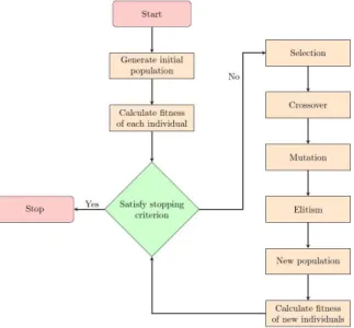
The algorithm used in this study is the popular genetic algorithm (GA). The GA was first introduced by Holland (1975) and since then various alterations were made (Baluja and Caruana, 1995; Janikow and Michalewicz, 1991). GAs are a form of evolutionary algorithms based on the mechanics of natural selection and natural genetics (Goldberg et al, 1989). A set of solutions called a population is initially generated and improved through iteration by means of three operators namely selection, crossover and mutation. Solutions may be encoded in different formats such as binary or real-valued encodings, which influence the techniques used for the operators, especially crossover.

The operators of a GA are applied sequentially on the population. First selection is applied to select a number of parent solutions which will be used to produce offspring solutions by means of crossover, which is a technique used to combine traits from the parent solutions to produce a number of offspring solutions. These operations are repeated until the next population is of the required size. In this study the elitism strategy (Baluja and Caruana, 1995) is also employed in the GA. The elitism strategy states that a predefined number of the best, in this case lowest weight, solutions that satisfies the constraints are automatically carried from one generation to the next. By using this strategy, it is ensured that a possible good solution is not lost through the iteration process. The procedure of the GA with elitism is outlined in figure 1.

(5)

4 IMPLEMENTATION

For the implementation of the GA along with functionality to optimize a structure with respect to size, shape and topology the MOEA Framework (Hadka, 2015) is used. This is an open source opti-mization framework written in the Java programming language. It provides a skeleton for implement-ing custom optimization problems, algorithms and variation strategies, while already housimplement-ing some of the most popular algorithms and variation strategies.

Our simple GA with elitism was added to the MOEA framework as well as a problem instance for each optimization approach used in this investigation.

Since each optimization approach is different in nature, different variables were used to define each of them and also different settings to allow for easy adaptation form one structure to the next.

Integer variables were used for sizing variables which can be encoded into binary strings. These integer variables range from zero to one less than the number of possible sections. The corresponding section can then be obtained by using the variable value as the index in the sorted list containing all the available cross-sections. The list is sorted according to ascending area size. By using the indices of the section rather than the actual list of sections, the built-in functionality of the MOEA Frame-work can be used to avoid creating new variables for real-valued discrete variables. In order to allow for symmetry in structures, functionality is also provided to allow for grouping of elements. Grouping mainly states that some structural elements have the same cross-section. Applying grouping reduces the number of variables of the problem and promotes uniformity in the structure.

The topology approach proved to be the simplest to implement in terms of variables. Boolean variables native to the MOEA Framework were used to indicate whether a member is present in a structure or not. This can be used with the ground structure approach (Dorn et al, 1964) where the initial structure contains all the possible elements and elements are eliminated as the optimization routine progresses. The option is also provided to select which members can be removed. By doing so allowance is made to ensure critical members will be present in all candidate structures. These may include members which are located at supports or directly carry a load. By utilising this setting the performance of the optimization routine can be greatly improved since the existence of solutions which will certainly not be feasible are inherently eliminated.

(6)

One important aspect of the generating of candidate solutions is the stability of the structure. For any trial structure the possibility exists that the structure is not stable. This may be due to unconnected members or internal mechanisms. One method to check the stability of a structure is to examine its stiffness matrix. If there are at any position on the matrix’s diagonal zero entries the structure can be deemed unstable. Unstable structures are usually an occurrence in problems where topology is being optimized. The check is then performed to avoid errors when trying to analyse unstable structures.

A total of seven optimization routines were used in this study. These include the three individual approaches, size, shape and topology, along with three staged routines. The first entails topology followed by size optimization (TS), the second starts with size, followed by topology and concludes with shape optimization (STS) and the third is a topology optimization, followed by shape and con-cluded with size optimization (TSS). The last routine is a simultaneous (SIM) optimization routine where size, shape and topology are considered at the same time.

5 NUMERICAL TESTS

This section is devoted to defining and comparing the results for various benchmark problems found in literature. All problems are solved using all seven routines and the recorded results are presented. These test problems include both 2D and 3D truss structures.

To obtain reliable results ten independent runs were executed. From these runs the average time and the best resulting structure are used in the presented results. This is required seeing as the result obtained from a heuristic search algorithm may deviate for each run.

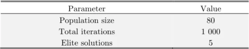
The same GA parameters are applied to all of the problems. These parameters are outlined in table 1. In the case of staged optimization, TS, STS and TSS, the number of iterations are divided to allow an acceptable amount for each stage. The transition from one stage to the next must also be defined. In this study, the transition is performed by taking the best solution from the previous stage as a template for the next stage. For instance, if a size routine must succeed a topology routine, the size routine will use the best topology found by the topology optimization routine and generate a new population by randomly initialising the cross-sections for the specific truss.

Parameter Value

Population size 80

Total iterations 1 000

Elite solutions 5

Table 1: Parameters used for the GA.

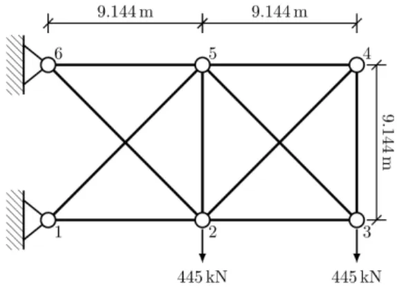
5.1 10-Bar Truss

(7)

Figure 2: 10-bar truss.

Parameter Value

Young’s modulus 68.95 GPa

Material density 2768 kg/m3

Allowable compressive stress 172.25 MPa

Allowable tensile stress 172.25MPa

Allowable displacement 50.8 mm

Table 2: 10-bar truss design parameters.

For this optimization problem, the selection of variables is fairly simple. All the elements are regarded as size and topology variables. For the shape optimization approach, the nodes on the bot-tom chord of the truss cannot move, while the nodes on the top chord can move in the vertical direction as defined in expression 2. This results in the problem consisting of ten size and topology variables with 3 shape variables.

4

5 6

5.0 25.0 5.0 25.0 5.0 25.0

m y m

£ £

(2)

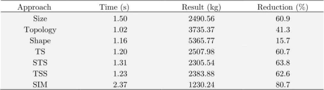
The results of the various optimization approaches are shown in table 3. The execution time along with the percentage of reduction from the base structure is also indicated. The weight of the base structure is determined from assigning the largest cross-section to all the members and calculating the weight of the structure.

This weight was determined as 6367 kg. In the table, some of the approaches are abbreviated with TS, STS, TSS and SIM referring to topology optimization followed by size optimization, size optimization followed by topology and shape optimization, topology followed by shape and size opti-mization and simultaneous size, shape and topology optiopti-mization respectively.

(8)

approach, the GA’s result of 1230kg compares well to those of 1282kg and 1235kg obtained by Tang et al (2005) and Rahami et al (2008) respectively.

Approach Time (s) Result (kg) Reduction (%)

Size 1.50 2490.56 60.9

Topology 1.02 3735.37 41.3

Shape 1.16 5365.77 15.7

TS 1.20 2507.98 60.7

STS 1.31 2305.54 63.8

TSS 1.23 2383.88 62.6

SIM 2.37 1230.24 80.7

Table 3: 10-bar truss results.

These comparisons indicate that the algorithm selected for this study provides reasonable results. Therefore, the algorithm can be regarded as an average performing optimization routine which makes it eligible for being used in a quantitative comparison study. It is important to ensure the same algorithm is used for all test problems and that it does not favour any of the seven routines.

The optimized structure resulting from the simultaneous optimization approach is shown in figure 3. The figure shows the resulting topology along with how the nodes were moved in order to produce the resulting structure. Since no elements are connected at node 4, it has subsequently been removed.

Figure 3: 10-Bar truss simultaneous optimization result.

(9)

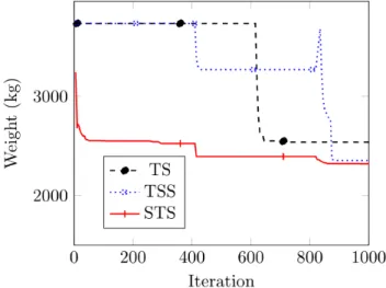
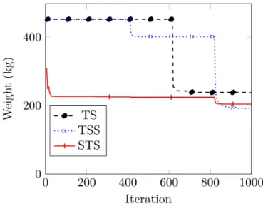
figure 4. The maximum number of iterations is shown in figure 5 to illustrate what happens when the transition is made from one stage to another during the execution of the respective routines. These transitions may be observed as the steps in the graphs at either 400, 600 or 800 iterations.

Figure 4: Performance of the size and simultaneous approaches for the 10-bar truss.

Figure 5: Performance of the TS, STS and TSS approaches for the 10-bar truss.

(10)

The topology and shape optimization routines are not shown in the figures due to their relatively poor performance with respect to the others. From the results, thus far the initial statement can be made that the shape and topology optimization routines does not perform well as single approaches. However, they do allow for improvement when used in conjunction with other strategies.

The weak performance of these two approaches may be attributed to their respective limitations. For example, topology optimization may only remove elements in the structure. In the case of the structure only having 10 elements, the number of elements that can be removed before the structure becomes unstable becomes very small. This limitation may be reduced in more complicated structures. A similar argument can be made for the shape optimization approach, the nodes that can vary in coordinates will only reduce the weight if the length of elements are reduced. Along with the pre-defined constraints of these nodes, the effectiveness of this approach is quite limited.

The behaviour of the TSS routine is interesting in this problem. On the transition from shape to size optimization the random initialization of the size variables causes an increase in the weight of the structure. This weight is then reduced to produce a good end result by the size optimization.

5.2 25-Bar Truss

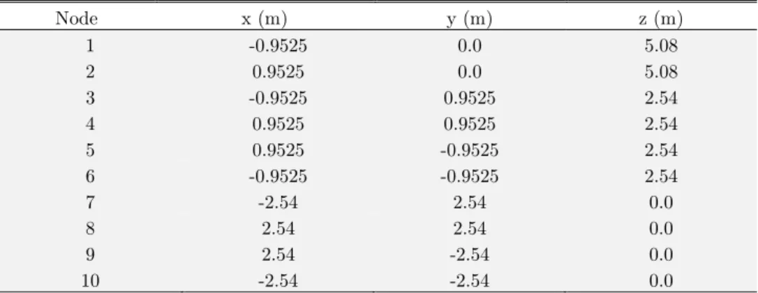
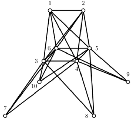
The first three-dimensional structure presented is the 25-bar space truss shown in figure 6. The prob-lem definition was taken from Schmit (1974) with the nodal coordinates listed in table 4 and the design parameters listed in table 7. The element information along with the grouping of elements is shown in table 6 and the loading conditions applied to the structure is shown in table 5.

Node x (m) y (m) z (m)

1 -0.9525 0.0 5.08

2 0.9525 0.0 5.08

3 -0.9525 0.9525 2.54

4 0.9525 0.9525 2.54

5 0.9525 -0.9525 2.54

6 -0.9525 -0.9525 2.54

7 -2.54 2.54 0.0

8 2.54 2.54 0.0

9 2.54 -2.54 0.0

10 -2.54 -2.54 0.0

Table 4: 25-bar truss nodal coordinates.

Node Fx (kN) Fy (kN) Fz (kN)

1 4.4482 -44.4822 44.4822

2 0 44.4822 44.4822

3 2.2241 0 0

6 2.6689 0 0

(11)

Group Element name (end nodes)

A1 1(1,2)

A2 2(1,4), 3(2,3), 4(1,5), 5(2,6)

A3 6(2,5), 7(2,4), 8(1,3), 9(1,6)

A4 10(3,6), 11(4,5)

A5 12(3,4), 13(5,6)

A6 14(3,10), 15(6,7), 16(4,9), 17(5,8)

A7 18(3,8), 19(4,7), 20(6,9), 21(5,10)

A8 22(3,7), 23(4,8), 24(5,9), 25(6,10)

Table 6: 25-bar truss element information.

Parameter Value

Allowable tensile stress 275.79 MPa

Only a few nodes are stipulated to form part of the five shape variables. Furthermore, grouping is used to reduce the amount of size and topology variables to only eight. These decisions force the structure to stay symmetrical. The detail regarding shape variables is shown in table 8.

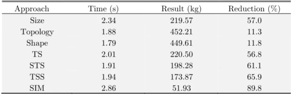
The optimization routines were executed for the seven approaches and the results obtained are summarised in table 9. Again, the abbreviations TS, TSS, STS and SIM refer to topology followed by size optimization, topology followed by shape and size optimization, size optimization followed by topology and shape optimization and simultaneous optimization respectively. The heaviest possible structure from assigning the biggest section weighed in at 510 kg.

(12)

Variable Detail

Shape variables (mm)

0.508 ≤ x4 ≤ 1.524 1.016 ≤ y4 ≤ 2.032 2.286 ≤ z4 ≤ 3.302 1.016 ≤ x8 ≤ 2.032 2.54 ≤ y8 ≤ 3.556

Symmetry

x4 = x5 = −x3 = −x6 y4 = y3 = −y5 = −y6

z4 = z3 = z5 = z6 x8 = x9 = −x7 = −x10

y8 = −y9 = −y10

Table 8: 25-bar truss variable detail.

Size 2.34 219.57 57.0

Topology 1.88 452.21 11.3

Shape 1.79 449.61 11.8

TS 2.01 220.50 56.8

STS 1.91 198.28 61.1

TSS 1.94 173.87 65.9

SIM 2.86 51.93 89.8

The performance of the approaches is shown in figures 7 and 8. By comparing figures 4 and 7 it can be seen that the performance of the approaches is fairly similar. It is also worth noting the 5 % difference between the results of the STS and TSS approaches. This indicates that their results are almost equivalent with the main difference being the starting weights of the routines. Where the TSS starting structure has the same cross-section assigned to all the elements and the STS’s start structure being randomly initialized.

(13)

As a validity check of the results obtained, they can be compared to the ones presented in litera-ture. For the size optimization approach, Dalolu (2008) and Coello et al (1994) arrived at 219.3 kg and 224 kg respectively, which correlates well with the 219.6 kg found in this study. When considering the simultaneous approach the 51.93 kg obtained is comparable to 50.7 kg found by Mortazavi and Toğan (2016).

5.3 47-Bar Truss

The next structure used is the two-dimensional 47-bar truss shown in figure 9 with the element definitions given in table 10. This problem has been used by a number of researchers to test their developed algorithms (Mortazavi and Toğan, 2016; Ahrari et al, 2015; Erbatur, 2002).

Element name (start node, end node)

A1 (1,3) A10 (6,8) A19 (10,11) A28 (14,16) A37 (15,17) A46 (5,6)

A2 (2,4) A11 (6,7) A20 (9,12) A29 (19,21) A38 (16,18) A47 (3,4)

A3 (2,3) A12 (5,8) A21 (11,13) A30 (20,22) A39 (14,21)

A4 (1,4) A13 (7,9) A22 (12,14) A31 (15,19) A40 (13,22)

A5 (3,5) A14 (8,10) A23 (12,13) A32 (16,20) A41 (21,22)

A6 (4,6) A15 (7,10) A24 (11,14) A33 (15,21) A42 (13,14)

A7 (4,5) A16 (8,9) A25 (13,21) A34 (16,22) A43 (11,12)

A8 (3,6) A17 (9,11) A26 (14,22) A35 (17,19) A44 (9,10)

A9 (5,7) A18 (10,12) A27 (13,15) A36 (18,20) A45 (7,8)

(14)

What makes this problem interesting is that there is no displacement constraint. However, an additional buckling constraint (equation 3) along with differing allowable tensile and compression stresses are imposed on this problem. These constraints along with other design parameters are shown in table 11.

2 / with 1,..., 47

3.96 i

comp BEA Li i

B

s £

= =

(3)

Parameter Value

Young’s modulus 206 84 GPa

Allowable tensile stress 137.9 MPa

(15)

Case Node Fx (kN) Fy (kN)

1 17, 18 26.69 -62.28

2 17 26.69 -62.28

3 18 26.69 -62.28

Table 12: 47-bar truss loading conditions.

Symmetry about the y-axis is preserved in the structure by means of prescribing opposing nodes to have the same value while it’s counterpart is allowed to be a shape variable during the optimization routines. These variables are shown in table 13. In total this problem consists of 27 size and topology variables and 17 shape variables which is significantly more than the previous two problems.

The results obtained from the various approaches are shown in table 14. The initial structure had a weight of 2989 kg and this was significantly reduced with the different optimization routines. The performance of the various optimization routines is shown in figures 10 and 11.

Figure 10: Performance of the size and simultaneous approaches for the 47-bar truss.

(16)

Variable Detail

Size and topology

Am = Am-1 With m = 2, 4, 6, …, 40

A41, A42, A43, …, A47

Shape variables (mm)

0 ≤ x2, x4, x6, x8 ≤ 3810 0 ≤ x10, x12, x14 ≤ 2286

0 ≤ x20 ≤ 3810 0 ≤ x22 ≤ 2286 0 ≤ y4 ≤ 6096 3084 ≤ y6 ≤ 9144 6096 ≤ y8 ≤ 10668 9144 ≤ y10 ≤ 12192 10668 ≤ y12 ≤ 13716 12192 ≤ y14 ≤ 15240 13716 ≤ y20, y22 ≤ 16764

Symmetry

x2 = -x1 ; x4 = -x3 x6 = -x5 ; x8 = -x7 x10 = -x9 ; x12 = -x11 x14 = -x13 ; x20 = -x19

x22 = -x21 y4 = y3 ; y6 = y5 y8 = y7 ; y10 = y9 Y12 = y11 ; y14 = y13 Y20 = y19 ; y22 = y21

Table 13: 47-bar truss variable detail.

Size 12.41 1381.66 53.8

Topology 11.00 2683.97 10.2

Shape 16.68 2407.19 19.5

TS 12.16 1422.37 52.4

STS 13.26 1420.75 52.5

TSS 15.16 1322.23 55.8

SIM 18.94 909.48 68.6

The resulting structure obtained from the simultaneous optimization had a weight of 909kg. This value is 8.7 % more than the 837kg from Gholizadeh (2013) and 13.5 % more than the 801kg reported by Mortazavi and Toğan (2016). The resulting weight difference between these papers may be at-tributed to the use of a better suited algorithm for a larger search space for the continuous shape variables.

(17)

of iterations. This indicates that there is an additional cost involved when optimizing a structure simultaneously as opposed to a staged approach.

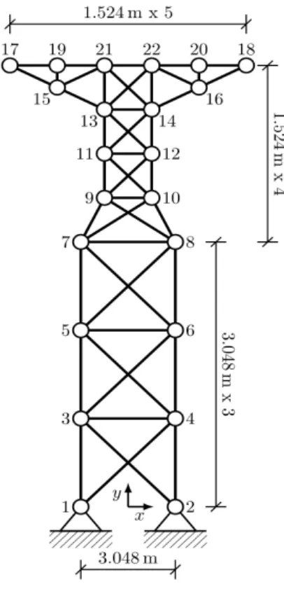
5.4 72-Bar Truss

The 72-bar space truss, shown in figure 12, was optimized for size and topology by Kaveh (2013) by applying both static and dynamic constraints. In this case, only static constraints are applied, but the shape of the structure is also optimized.

Figure 12: 72-Bar truss.

The design parameters along with the displacement and stress constraints used in this problem are shown in table 15. With the element grouping for the 16 size and topology variables as detailed in table 16. The list of 64 cross-sections used for this problem was taken from Kaveh et al (2016).

Parameter Value

Allowable stress 172.38 MPa

Table 15: 72-bar truss design parameter.

The structure is also subjected to two load cases. Each applying a different stress pattern within the structure. These load cases are specified in table 17.

(18)

Group Element name (end nodes)

A1 1(1,5), 2(2,6), 3(3,7), 4(4,8)

A2 5(2,5), 6(1,6), 7(2,7), 8(3,6), 9(3,8), 10(4,7), 11(1,8), 12(4,5)

A3 13(5,6), 14(6,7), 15(7,8), 16(5,8)

A4 17(5,7), 18(6,8)

A5 19(5,9), 20(6,10), 21(7,11), 22(8,12)

A6 23(6,9), 24(5,10), 25(6,11), 26(7,10), 27(7,12), 28(8,11), 29(5,12), 30(8,9)

A7 31(9,10), 32(10,11), 33(11,12), 34(9,12)

A8 35(9,11), 36(10,12)

A9 37(9,13), 38(10,14), 39(11,15), 40(12,16)

A10 41(10,13), 42(9,14), 43(10,15), 44(11,14), 45(11,16), 46(12,15), 47(9,16), 48(12,13)

A11 49(13,14), 50(14,15), 51(15,16), 52(13,16)

A12 53(13,15), 54(14,16)

A13 55(13,17), 56(14,18), 57(15,19), 58(16,20)

A14 59(14,17), 60(13,18), 61(14,19), 62(15,18), 63(15,20), 64(16,19), 65(13,20), 66(16,17)

A15 67(17,18), 68(18,19), 69(19,20), 70(17,20)

A16 71(17,19), 72(18,20)

Table 16: 72-bar truss grouping.

Case Node Fx (kN) Fy (kN) Fz (kN)

1 17 22.25 22.25 -22.25

2 17, 18, 19, 20 0 0 -22.25

Table 17: 72-bar truss loading conditions.

The results from the various optimization routines is given in table 18. The base structure used has a weight of 626.9 kg. This is not the heaviest structure possible from the selection of sections, but given the large range of section sizes and the results obtained a lighter structure which also satisfies the constraints was selected for the comparison.

Size 10.30 216.72 65.4

Topology 9.12 446.23 28.8

Shape 9.06 402.20 35.8

TS 9.83 216.79 65.4

STS 8.95 164.21 73.8

TSS 9.5 143.69 77.1

SIM 11.97 97.58 84.4

(19)

172 kg which compares well with the other papers. Unfortunately, to the authors’ knowledge, no results to the simultaneous approach have been published for the 72-bar truss and the results obtained in this study can therefore not be compared to ones from literature.

The performance of the individual routines is shown in figures 13 and 14.

Figure 13: Performance of the size and simultaneous approaches for the 72-bar truss

6 CONCLUSION

(20)

considered include the individual size, shape and topology optimization techniques along with three staged combinations and a simultaneous approach.

Only truss structures were considered and the weight of the structure, which can be related to cost, was used as the objective of the optimization. The validity of the results obtained by the GA was established by comparing some of the resulting weights with those available in literature. The performance of these seven routines was measured by comparing the time required for the routine to run as well as the percentage of weight saving relative to a base structure. A total of four structures were tested.

From the result obtained in this study, the well-known statement that considering the size, shape and topology aspects of the structure simultaneously produces the lightest structures is validated. Through the quantification used in this study it can be concluded that the simultaneous approach yields, on average, a 13 % better solution than its best alternative, but requires additional computational time to complete.

Between the individual approaches, size optimization clearly leads to the better results, but consumes more time. From the results obtained in this study the weight improvement is about 32 %. The reason for this can be attributed to the fact that the choice of cross-section has a significant influence on the weight of the structure, while removing certain non-critical elements and moving joins can only influence the weight of the structure to a lesser extent.

The staged approaches typically produce reasonable results with the same amount of iterations. However, the iterations allowed for each stage are quite limited when each routine is to have the same total number of iterations. It is interesting to note that there is on average a 12 % difference between considering all the three aspects in a staged manner as opposed to considering them simultaneously. The separation of the size, shape and topology aspects of the structure may be the cause for this difference since these aspects are not independent when it comes to the performance of the structure. It is possible to quantify from the results in this study that the simultaneous approach produces, on average, 22 % more economical structures than the size approach. It also always arrives at a better result than any of the considered staged approaches. This indicates that in search of a truly optimal structure, simply performing a size optimization is insufficient and that significant savings in terms of weight can be made by upgrading the optimization routine’s complexity by considering more as-pects of the structure.

References

Achtziger W (2007) On simultaneous optimization of truss geometry and topology. Structural and Multidisciplinary Optimization 33, DOI 10.1007/ s00158-006-0092-0

Ahrari A, Atai AA, Deb K (2015) Simultaneous topology, shape and size optimization of truss structures by fully stressed design based on evolution strategy. Engineering Optimization 47(8):1063–1084, DOI 10.1080/0305215x.2014.947972

Baluja S, Caruana R (1995) Removing the genetics from the standard genetic algorithm. In: Machine Learning: Pro-ceedings of the Twelfth International Conference, pp 38–46, DOI 10.1016/b978-1-55860-377-6.50014-1

Bendsøe, MP, Ben-Tal A, Zowe J (1994) Optimization methods for truss geometry and topology design. Structural and Multidisciplinary Optimization 7, DOI 10.1007/ bf01742459

(21)

Camp CV, Bichon BJ (2004) Design of space trusses using ant colony optimization. Journal of Structural Engineering 130(5):741–751, DOI 10.1061/(asce) 0733-9445(2004)130:5(741)

Coello CC, Rudnick M, Christiansen AD (1994) Using genetic algorithms for optimal design of trusses. In: Tools with Artificial Intelligence, 1994. Proceedings., Sixth International Conference on, IEEE, pp 88–94, DOI 10.1109/tai. 1994.346509

Degertekin M SO; Hayalioglu (2013) Sizing truss structures using teachinglearning-based optimization. Computers & Structures 119, DOI 10.1016/j. compstruc.2012.12.011

Dorn WS, Gomory RE, Greenberg HJ (1964) Automatic design of optimal structures. Journal de Mecanique 3:25–52, DOI 10.1016/b978-0-08-010580-2.50008-6

Erbatur OHF (2002) On efficient use of simulated annealing in complex structural optimization problems. Acta Me-chanica 157, DOI 10.1007/bf01182153

Gholizadeh S (2013) Layout optimization of truss structures by hybridizing cellular automata and particle swarm optimization. Computers & Structures 125, DOI 10.1016/j.compstruc.2013.04.024

Goldberg DE, et al (1989) Genetic algorithms in search optimization and machine learning, vol 412. Addison-wesley Reading Menlo Park, DOI 10.5860/choice. 27-0936

Hadka D (2015) Moea framework - a free and open source java framework for multiobjective optimization. version 2.11. URL http://www.moeaframework.org

Holland, J.H., 1975. Adaptation in natural and artificial systems. An introductory analysis with application to biology, control, and artificial intelligence. Ann Arbor, MI: University of Michigan Press.

Jalili S, Hosseinzadeh Y (2015) A cultural algorithm for optimal design of truss structures. Latin American Journal of Solids and Structures 12(9):1721–1747, DOI 10.1590/1679-78251547

Janikow CZ, Michalewicz Z (1991) An experimental comparison of binary and floating point representations in genetic algorithms. In: ICGA, pp 31–36, DOI 10.1007/bf01889983

Kaveh A A; Zolghadr (2013) Topology optimization of trusses considering static and dynamic constraints using the css. Applied Soft Computing 13, DOI 10.1016/j.asoc.2012.11.014

Kaveh A, Kalatjari VR, Talebpour MH (2016) Optimal design of steel towers using a multi-metaheuristic based search method. Periodica Polytechnica Civil Engineering 60(2):229–246, DOI 10.3311/ppci.8222

Kaveh A, Talatahari S (2009) Size optimization of space trusses using big bang– big crunch algorithm. Computers & structures 87(17):1129–1140, DOI 10.1016/ j.compstruc.2009.04.011

Kocvara M, Zowe J (1996) How mathematics can help in design of mechanical structures. Preprint 171, Institut fr Agewandte Mathematik, Universitt Erlangen-Nrnberg, URL http://www.math.fau.de/fileadmin/preprints/pr171.html Luh GC, Lin CY (2011) Optimal design of truss-structures using particle swarm optimization. Computers & Structures 89, DOI 10.1016/j.compstruc.2011.08.013

Miguel LFF, Lopez RH, Miguel LFF (2013) Multimodal size, shape, and topology optimisation of truss structures using the firefly algorithm. Advances in Engineering Software 56:23–37, DOI 10.1016/j.advengsoft.2012.11.006

Mohr DP, Stein I, Matzies T, Knapek CA (2011) Robust topology optimization of truss with regard to volume. arXiv preprint arXiv:11093782 DOI 10.1007/ s11081-013-9241-7

Mortazavi A, Toğan V (2016) Simultaneous size, shape, and topology optimization of truss structures using integrated particle swarm optimizer. Structural and Multidisciplinary Optimization pp 1–22, DOI 10.1007/s00158-016-1449-7 Nanakorn P, Meesomklin K (2001) An adaptive penalty function in genetic algorithms for structural design optimiza-tion. Computers & Structures 79, DOI 10.1016/s0045-7949(01)00137-7

(22)

Pederson N, Nielson A (2003) Optimization of practical trusses with constraints on eigenfrequencies, displacements, stresses, and buckling. Structural and Multidisciplinary Optimization 25, DOI 10.1007/s00158-003-0294-7

Rahami H, Kaveh A, Gholipour Y (2008) Sizing, geometry and topology optimization of trusses via force method and genetic algorithm. Engineering Structures 30(9):2360–2369, DOI 10.1016/j.engstruct.2008.01.012

Schmit B LA; Farshi (1974) Some approximation concepts for structural synthesis. AIAA Journal 12, DOI 10.2514/3.49321

Sivakumar P, Rajaraman A, Samuel Knight G, Ramachandramurthy D (2004) Object-oriented optimization approach using genetic algorithms for lattice towers. Journal of computing in civil engineering 18(2):162–171, DOI 10.1061/(asce) 0887-3801(2004)18:2(162)

Sobieszczanski-Sobieski J, James BB, Riley MF (1987) Structural sizing by generalized, multilevel optimization. AIAA Journal 25, DOI 10.2514/3.9593

Stolpe M (2016) Truss optimization with discrete design variables: a critical review. Structural and Multidisciplinary Optimization 53(2):349{374, DOI 10.1007/ s00158-015-1333-x, URL http://dx.doi.org/10.1007/s00158-015-1333-x Tang W, Tong L, Gu Y (2005) Improved genetic algorithm for design optimization of truss structures with sizing, shape and topology variables. International Journal for Numerical Methods in Engineering 62(13):1737–1762, DOI 10.1002/nme.1244

Toan V, Dalolu AT (2008) An improved genetic algorithm with initial population strategy and self-adaptive member grouping. Computers & Structures 86, DOI10.1016/j.compstruc.2007.11.006