Setembro, 2016 Vasco da Silva Brito

(1)

1

S e te m b ro , 2016 Va s c o d a S ilva Brito

Lice ncia do e m Ciê ncia s da Enge nha ria Ele troté cnica e de Computa dore s

Fa u lt To le ra n t Co n tro l o f a X8-VB Qu a d c o p te r

Dis s e rta çã o pa ra Obte nçã o do Gra u de Me s tre e m Enge nha ria Ele troté cnica e de Computa dore s

Orie nta dor: Luís Filipe Figue ira Brito P a lma , P rofe s s or Auxilia r, Fa culda de de Ciê ncia s e Te cnologia da Unive rs ida de Nova de Lis boa

J úri:

P re s ide nte : J oã o Alme ida da s Ros a s , P rofe s s or Auxilia r, FCT-UNL

Argue nte : Albe rto J orge Le bre Ca rdos o, P rofe s s or Auxilia r, FCT-UC

Voga l: Luís Filipe Figue ira Brito P a lma , P rofe s s or Auxilia r, FCT-UNL

(2)

(3)

iii Fault Tolerant Control of a X8-VB Quadcopter

(4)

(5)

v

(6)

(7)

vii

Acknowledgments

The realization of this thesis represents the end of an adventure, one more important step in my life. I would like to thank all who participated directly and indirectly to fulfill this journey with success.

First of all, I would like to thank my advisor Professor Luís Filipe Figueira Brito Palma for the opportunity, transmitted knowledge, patience and friendship. I would also like to thank him for the unconditional support and confidence, as well as for the provided working condition and tools.

I would also like to show gratitude my colleagues and friends, Afonso Maria, André Quintanova, Alexandre Brito, Guilherme Almeida, Liliana Sequeira, Rui Barrocas, Rui Antunes, Tiago Santos, Yaniel Barbosa among others for the unconditional support and friendship. Similarly, to my mentees, Miguel Pita, Luís Alves and Marcos Estrela, special thanks for the effort made during the programs.

Special thanks to my friends Ana Areias, Catarina Martins, Ricardo Bettencourt and Samuel Meneses for helping me unwind from time to time when I needed.

A profound acknowledgment to my family for the strength, protection and dedication provided along these years. To my parents, Carlos and Alda Brito for helping me grow into what I am today and for the sacrifices made in offspring of my education and professional formation. I would also like to recognize my uncle Paulo Brito, my aunt Benvinda Brito and my cousins Carolina and Ana Sofia Brito for having me every Sunday for lunch (sometimes for diner too), for our constructive discussions about every kind of subject and for the good advices.

(8)

(9)

ix

Abstract

In this dissertation new modeling and fault tolerant control methodologies of a quadcopter with X8 conﬁguration are proposed; studies done to actuators faults and possible reconfigurations are also presented.

The main research effort has been done to design and implement the kinematic and dynamic model of a quadcopter with X8 configuration in Simulink®. Moreover, simulation and control of the quadcopter in a virtual reality world using Simulink3D® and real world experimental results from a quadcopter assembled for this purpose.

The main contributions are the modeling of a X8 architecture and a fault tolerant control approach. In order to show the performance of the controllers in closed-loop, simulation results with the model of a X8 quadcopter and real world experiments are presented.

The simulations and experiments revealed good performance of the control systems due to the aircraft model quality. The conclusion of the theoretical studies done in the field of actuators’ fault tolerance were validated with simulation and real experiments.

(10)

(11)

xi

Resumo

Nesta dissertação propõem-se novas metodologias de modelização e controlo tolerante a falhas de um quadcopter com configuração X8; apresentando-se estudos realizados com falhas em atuadores e estratégias de reconfiguração.

O maior esforço de investigação foi despendido na conceção e implementação dos modelos cinemático e dinâmico de um quadcopter com a configuração X8 em Simulink®. As tarefas posteriores foram a simulação e o controlo do quadcopter num mundo de realidade virtual usando Simulink3D® e a obtenção de resultados experimentais do mundo real a partir de um quadcopter montado para esse fim.

As principais contribuições são a modelação de um quadcopter com arquitetura X8 e uma abordagem de controlo tolerante a falhas. A fim de mostrar o desempenho dos controladores em anel fechado, apresentam-se resultados das simulações com o modelo de um quadcopter X8 e resultados experimentais no mundo real.

As simulações e as experiências revelaram um bom desempenho dos sistemas de controlo devido à boa qualidade do modelo proposto para a aeronave. As conclusões do estudo teórico realizado na área de tolerância a falhas nos atuadores foram validadas em simulações e em testes reais.

Palavras-chave: quadcopter, modelação, tolerância a falhas, controlo tolerante a

(12)

(13)

xiii

Notations and Symbols

Notations

ARX: auto-regressive linear model with exogenous input

CCW: counter-clock wise

CW: clock wise

DC: direct current

ESC: electronic speed controller

FDD: fault detection and diagnosis

FTC: fault tolerant control

LiPo: lithium polymer

MRAS: model reference adaptive systems

PID: proportional-integral-derivative

PSO: particle swarm optimization

PWM: pulse wide modulation

RPM: rotations per minute

SMC: sliding mode controller

SPE: solid polymer electrolyte

STR: self-tuning regulator

TDM: time division multiplexing

(14)

xiv Symbols and Operators

Variables and scalars are represented by small letters in italic, (ex. 𝑥(𝑡), 𝑎, …). Matrices are represented by capital letters in bold, (ex. 𝑴, 𝑴(: , : , 𝑘), …). Vectors are represented in small letters, in bold, (ex., x(:,k), y, …).

t Continuous time variable

k Discrete time variable

x(t) Continuous time signal at instant t

x(k) Discrete time signal at discrete time k

𝑇𝑠 Sampling time

g Gravity acceleration

m Body mass

e Control error

v Temporary control actuation

u Control saturated actuation

𝑈𝑛 Sum of motors’ forces

ϕ, θ, ψ Roll, pitch and yaw, respectively

𝑓𝑛 Motor’s force

ω𝑛 Motor’s rotation speed (rad/s)

m Mass (Kg)

l Length (m)

h Height (m)

r Radius (m)

sat() Saturation function

mse() Mean square error function

(15)

xv

List of Figures

Figure 1.1 - Thesis workflow diagram. ... 2

Figure 2.1 - Breguet-Richet Gyroplane. ... 6

Figure 2.2 - Oehmichen No.2 aircraft. ... 7

Figure 2.3 – Convertawings, Inc. Model A Quadrotor. ... 7

Figure 2.4 – Faraday’s electromagnetic experiment, 1821. ... 8

Figure 2.5 - a) Archimedes' screw; b) Leonardo da Vinci's draw. ... 9

Figure 2.6 - Wright Brothers' propeller. ... 10

Figure 2.7 - History of ionic conductivity improvements. ... 11

Figure 2.8 - Closed-loop system simulation with proportional control. ... 13

Figure 2.9 - Closed-loop system simulation with PI control. ... 14

Figure 2.10 - Closed-loop system simulation with PID control. ... 15

Figure 2.11 - Fuzzy controller architecture. ... 15

Figure 2.12 - Example of membership functions... 16

Figure 2.13 - Sliding mode in a second order relay system. ... 18

Figure 2.14 - Discretization example. ... 19

Figure 2.15 - Generic adaptive control diagram. ... 21

Figure 2.16 - Block diagram of a system with gain scheduling. ... 22

Figure 2.17 - Block diagram of a MRAS ... 23

(20)

xx

Figure 2.19 - Generic supervisory diagram. ... 25

Figure 2.20 - Categories of faults in a system. ... 27

Figure 2.21 – Two dimensional performance regions. ... 28

Figure 2.22 - Fault types regarding temporal behavior ... 29

Figure 2.23 - Fault tolerant control architecture. ... 30

Figure 2.24 - Reconfiguration control in response to a fault. ... 31

Figure 2.25 - Samir Bouabdallah’s micro-quadcopter. ... 34

Figure 2.26 – Sérgio Costa’s prototype. ... 34

Figure 2.27 - José Sousa’s Quadcopter. ... 35

Figure 2.28 - Images from Mellinger’s experimental trials.. ... 35

Figure 3.1 - Workflow diagram. ... 37

Figure 3.2 - High level hardware architecture. ... 38

Figure 3.3 – 3D model of upper and lower sides of the adapter. ... 39

Figure 3.4 – 3D model of the extension piece. ... 39

Figure 3.5 - Complete 3D model. ... 40

Figure 3.6 - Simplified 3D model. ... 40

Figure 3.7 - Weight and dimension related to power density ... 41

Figure 3.8 - On the left, the 6000 mAh battery. On the right, the 5000 mAh battery. .... 42

Figure 3.9 – Radio Frequency communication device. ... 43

Figure 3.10 - Arduino Due and 3DR pin connections. ... 44

Figure 3.11 – FrSky Taranis X9D Plus on the right and the receiver on the left. ... 45

Figure 3.12 - Shield GPS Logger. ... 46

Figure 3.13 - 9-Axis Shield. ... 47

(21)

xxi

Figure 3.15 -ACS712 Current Sensor. ... 48

Figure 3.16 - ESC 420 Lite. ... 49

Figure 3.17 - BLDC motor ... 50

Figure 3.18 - Propeller rotation plot ... 51

Figure 3.19 - CCW propeller ... 51

Figure 3.20 - Representation of equal rotations and forces. ... 52

Figure 3.21 - Representation of a positive roll rotation forces. ... 54

Figure 3.22 - Representation of a positive pitch rotation forces... 55

Figure 3.23 - Representation of a positive yaw rotation forces. ... 56

Figure 3.24 – Earth referential (E), Aircraft referential (A) and position vector PE. ... 57

Figure 3.25 – Developed and implemented test bench. ... 68

Figure 3.26 - Motor and propeller experimental result. ... 69

Figure 3.27 – Two motors and propellers experimental result. ... 69

Figure 3.28 - Motor model step response. ... 70

Figure 3.29 - High-level control architecture. ... 72

Figure 3.30 – Low-level control architecture. ... 73

Figure 3.31 - PID with anti-windup architecture. ... 74

Figure 3.32 - Relay controller application to the altitude.. ... 76

Figure 3.33 - Ultimate sensitivity method applied to pitch rotation. ... 78

Figure 3.34 - Ultimate sensitivity method applied to yaw rotation. ... 79

Figure 3.35 - Block diagram example of the cascade control system. ... 80

Figure 3.36 - Ultimate sensitivity applied to the X variable. ... 81

Figure 3.37 - Trajectory with yaw rotation. ... 82

(22)

xxii

Figure 3.39 - Four motors quadcopter fault experiment. ... 89

Figure 3.40 - Reconfiguration due to motor 1 failure. ... 90 Figure 3.41 – Reconfiguration due to two motors failure (𝑓1 and 𝑓3). ... 91 Figure 3.42 - Absolute Orientation Sensor pitch/roll steady state data experiment. ... 94

Figure 3.43 - Absolute Orientation Sensor yaw steady state data experiment ... 94 Figure 3.44 - AltIMU steady state data experiment. ... 95 Figure 3.45 - Current sensor steady state response. ... 95

Figure 3.46 – ESC initialization function code. ... 96

Figure 3.47 – Example of ESC update function code. ... 96 Figure 3.48 - Example of discrete PID Arduino implementation. ... 97 Figure 3.49 – Example of SMC Arduino implementation. ... 97

Figure 4.1 – Altitude switching PID control simulation. ... 100

Figure 4.2 - Low altitude PID response simulation. ... 100 Figure 4.3 – Altitude PID actuation. ... 101

Figure 4.4 – Altitude motors’ response to the PID actuation. ... 101

Figure 4.5 - Pitch and roll independent simulation. ... 102 Figure 4.6 - PID actuation to pitch and roll. ... 102 Figure 4.7 - Motors' response for pitch and roll simulations... 103

Figure 4.8 – Pitch and roll simultaneous simulation. ... 104 Figure 4.9 - PID Yaw simulation. ... 105 Figure 4.10 - PID actuation for yaw rotation. ... 105

(23)

xxiii

Figure 4.14 - Trajectory PID controllers without yaw rotation. ... 108

Figure 4.15 - Trajectory PID controllers actuations and rotations response. ... 108 Figure 4.16 - Trajectory PID controllers with yaw rotation. ... 109 Figure 4.17 - Trajectory PID controllers actuations and rotations response. ... 109

Figure 4.18 – Yaw PID, based on PSO, simulation. ... 110 Figure 4.19 – PID, based on PSO, actuation for yaw rotation. ... 111 Figure 4.20 – PSO PID controllers without yaw rotation applied to trajectory. ... 112

Figure 4.21 - PSO PID controllers’ actuations and rotations response. ... 112

Figure 4.22 - Yaw SMC, based on PSO, simulation. ... 113 Figure 4.23 - SMC, based on PSO, actuation for yaw rotation. ... 113 Figure 4.24 - PSO SMC controllers without yaw rotation applied to trajectory. ... 114

Figure 4.25 - PSO SMC controllers’ actuations and rotations response. ... 114

Figure 4.26 – Position/trajectory tolerant fault control to motor 1 failure. ... 115 Figure 4.27 – Position/trajectory rotations fault tolerant control to motor 1 failure. ... 116

Figure 4.28 – Position/trajectory motors' response to motor 1 failure.. ... 116

Figure 4.29 – Position/trajectory FTC to motor 1 failure, safe landing.. ... 117 Figure 4.30 – Position/trajectory rotations FTC to motor 1 failure, safe landing. ... 117 Figure 4.31 – Position/trajectory motors' response to motor 1 failure.. ... 118

Figure 4.32 - Pitch experiment restrain configuration. ... 118 Figure 4.33 – Pitch sensor data received by the base station. ... 119 Figure 4.34 – Pitch PID control actuation. ... 119

(24)

xxiv

Figure 4.38 – Yaw PID control actuation. ... 121

Figure 4.39 - Attitude sensors data received by the base station. ... 122 Figure 4.40 - Attitude PID controllers’ actuation. ... 123 Figure 4.41 – Faulty attitude sensors data received by the base station. ... 124

(25)

xxv

List of Tables

Table 3.1 - Arduino DUE specifications (Source: Arduino)... 42

Table 3.2 - 3DR Radio V2 specifications. ... 44 Table 3.3 - Shield GPS Logger specifications ... 46 Table 3.4 - 9-Axis shield power specifications. ... 47

Table 3.5 - AltiMU power specifications. ... 47 Table 3.6 - Current sensor specifications. ... 48 Table 3.7 - ESC specifications. ... 49 Table 3.8 - BLDC specifications ... 50 Table 3.9 - Inertial calculations results. ... 67

Table 3.10 - Ziegler-Nichols Rules ... 75

Table 3.11 - Altitude PID gains. ... 77 Table 3.12 - Roll/Pitch PID gains. ... 78 Table 3.13 - Yaw PID gains. ... 79

Table 3.14 - X/Y PID gains. ... 81

Table 3.15 - PID controllers’ gains obtained from PSO algorithm. ... 86 Table 3.16 - SMC controllers’ gains obtained from PSO algorithm. ... 87

Table 3.17 - Motors failure and reconfigurations ... 92

(26)

xxvi

(27)

1

Chapter 1

1 Introduction

1.1 Motivation

The operation of aircrafts requires a good amount of expertise and, in today´s quest of finding the cheapest solution, the need of hiring an operator can increase the costs significantly. The current growth of interest in unmanned aircrafts has been changing the companies' world. The major problems regarding these kinds of subjects are the reliability and security of the aircrafts and the people. Over-actuated systems, as well as fault detection and diagnosis, are fascinating and complex topics, representing major research areas. Their application to unmanned aircrafts is just the tip of the iceberg involving different areas such as control, soft computing, digital image processing and much more.

This research is related with the fault diagnosis and fault tolerant control implemented in an over-actuated system. The control challenge and the security of aircraft and people led the author of this dissertation to work in this research field.

1.2 Main Goals and Contributions

(28)

2

The main goal of this dissertation is to focus on the detection of failures on the aircraft’s actuators corresponding to a quadcopter’s fault, designing fault tolerant controllers and apply them to a real world situation. Another objective is to assemble the quadcopter X8 design, in order to posteriorly apply the algorithms of fault tolerant control. Moreover, to create a model that represents the dynamic and kinematic of the aircraft and, with this, design the control algorithms. An additional intent is to develop a virtual reality world where the model dynamics and kinematics could be easily observed and explained to people.

This dissertation will follow the subsequent workflow diagram (Figure 1.1) where parallel activities are present.

Figure 1.1 - Thesis workflow diagram.

The main contribution is the use of fault detection applied to a real world aircraft using algorithms of control allocations, in order to allow an over-actuated multirotor to fulfill a mission under faulty conditions. Another contribution is the development of a kinematic and dynamic model allowing to better understand the dynamic behavior of aircrafts of this type and able to simulate faults/failures. In addition to these contributions, the model will contribute to the educational area, allowing students learn about aerodynamics.

1.3 Thesis structure

(29)

3

In Chapter 1, the motivation, the main goals, and contributions of the dissertation structure are presented.

Chapter 2 contains the state-of-the-art with background concepts used in the research, which come from diversified areas. These concepts are presented and discussed in this chapter.

Chapter 3 shows the research development, from the mathematical modelation of the dynamic and kinematic of the aircraft, through the motors and propellers modelation, until the final and most important topic arrives - the fault tolerant control technique developed.

In Chapter 4, simulations and experimental results of the fault tolerant control algorithms and other flight trials are presented here as well as a comparison between methods.

(30)

(31)

5

Chapter 2

2 State of the Art

2.1 Introduction

The state of the art will present and discuss all the main concepts used in this work. The ground work for this research came from different fields of study. Concepts can derive from DC motor or propellers to the physical modulation of a full functional quadcopter.

Notions like the origin of multirotors, DC motors, propellers as well as Proportional Integral Derivative (PID) controllers, Fuzzy logic, Sliding Mode Controllers (SMC), Fault Detection and Diagnosis (FDD) and over-actuated systems are briefly reviewed here.

(32)

6

2.2 Multirotors

2.2.1 History

Louis and Jacques Breguet invented the first quadrotor in France, with the supervision of Charles Richet, in 1907. It was the first piloted aircraft able the lift vertically. Originally, it was called gyroplane, now adapted to helicopter or multirotor. The design was very simple, as we can see in Figure 2.1. This was the first known attempt to build a quadrotor and it is known to have actually flown several times (Young, 1982).

Figure 2.1 - Breguet-Richet Gyroplane.

(33)

7

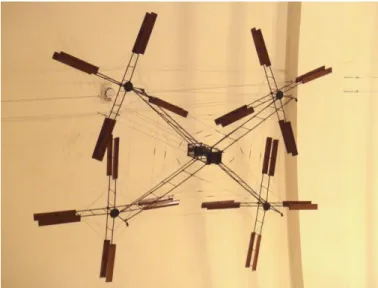
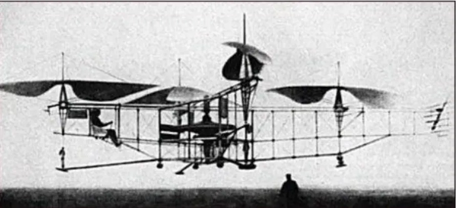
Figure 2.2 - Oehmichen No.2 aircraft.

The next important step in quadcopter history was a prototype made by Convertawings, Inc. in 1956 called Model A Quadrotor (Figure 2.3). The design had two engines driving four rotors, no tail rotor was needed, and the control was made by varying the thrust between the rotors, like nowadays quadcopters. It flew successfully many times and was the first quadrotor design able to forward flight reliably. Unfortunately, due to lack of commercial and military needs, the project was abandoned (Convertawings Inc, 1956).

Figure 2.3 – Convertawings, Inc. Model A Quadrotor.

(34)

8

2.2.2 DC Motors

The purpose of the electric motors is to convert electrical energy into mechanical energy. This is possible by interacting magnetic fields - one stationary and the other moving. DC motors are the simpler and older motors around, invented in the early 1820s. The design was possible after Oersted, Gauss and Faraday discovered the electromagnetic principles in the early 1800’s. In October of 1821, Faraday successfully confirmed the conversion of electrical energy into movement (Figure 2.4); the demonstration was published in the “Quarterly Journal or Science Literature, and the Arts” in 1822 (Royal Institution of Great Britain, 1822), being recognized as the inventor of the electrical motors concept (Qadir, 2013).

Figure 2.4 – Faraday’s electromagnetic experiment, 1821(Faraday, 1822).

Several years after Faraday’s experiment, Joseph Henry improved the design by building an electromagnet rotor that reversed automatically the polarity by its motion as pairs of wires made contact alternately with two cells; two permanent magnets create a flux that alternately attract and repel the electromagnets, making them go back and forth at 75 cycles per minute. Although it was only a lab experiment, it was more mechanically useful than Faraday’s early research. Joseph Henry’s design also showed that it was feasible to develop electrical generators and motors (Qadir, 2013).

Not long after Henry’s tryouts (1832), William Sturgeon invented the

(35)

9

After long years of evolution regarding DC motors, Brushless DC motors (BLDC) appeared in 1962, developed by T.G. Wilson and P.H. Trickey, which was called “CD Machine with Solid State Commutation” (Wilson & Trickey, 1962). In the beginning, the technology to make such a motor practical for industrial use did not exist. Only after the arrival of powerful magnet materials and high voltage transistors, in the early 1980’s, was the use of BLDC a possibility (Qadir, 2013). The key component differing BLDC and their predecessor’s most common used DC motors was the loss of an element, as the name suggests, the brushes. Without these, the efficiency of the motor increases, as well as the longevity, since the friction between the rotor and the brushes no longer exist. It also has a major advantage - because there is no need of sliding contacts, brushes or excitation windings, the BLDC react with promptness to variations in current, making them better at dynamic performance (Yedamale, 2003).

The exclusion of the brushes makes the motors easy to assemble and repair, as well as modifying the motors' construction, making them smaller and lighter. This progress also improves the speed contrasted with torque characteristic and can reach high speeds with less noise. Because of the construction design, the BLDC have high electrical efficiency (Yedamale, 2003) being the perfect match for drone use.

2.2.3 Propellers

The principal of a propeller is to convert rotation motion into propulsive force. The first known sketch of a propeller applied to airlift is from the Italian scientist Leonardo da Vinci, circa 1490 (Figure 2.5 b). It was a human-powered helicopter with no real-world application (Heatly, 1986). The propeller design in Leonardo’s drawing was inspired by Archimedes’ water screw invention (Figure 2.5 a).

(36)

10

The Wright Brothers engineered the aircraft propeller that we know today. By conducting experiments with wings in wind tunnels, they realized that propellers had essentially the same shape and behavior as wings (Figure 2.6). They also realized that a twist along the length of the blade was needed in order to keep the angle of attack uniform alongside all the extension of the propeller (Crouch, 2004).

Figure 2.6 - Wright Brothers' propeller (Kaempffert, 1911).

The design of propellers has the angle of attack as a major effectiveness factor. As the Wright Brothers discovered, the angle of attack needs to be constant along the length of the propeller’s blade, eliminating the possibility of stall. Another significant factor of effectiveness is the pitch. It is defined by the distance travelled in one revolution. These two factors allow the measurement of the efficiency of propellers (Federal Aviation Administration, 2008).

2.2.4 Energy Power Source

(37)

11

There are three types of SPEs: dry SPE, gelled SPE and porous SPE. Michel Armand first used the dry SPE in prototype batteries around 1978 (M.B. Armand, J.M. Chabagno, 1978). Later (1985), other companies used dry SPEs like ANVAR and Elf V Acquitaine from France, as well as Canadians’ Hydro Quebec. The gelled SPEs were used some years later, around the 1990s, by several organizations like Mead and Valence from The United States and GS Yuasa in Japan. Although the American Bellcore started commercialization of rechargeable LiPo cells using porous SPE, the business was not successful (Murata, Izuchi, & Yoshihisa, 2000). The historical evolution can be observed in Figure 2.7.

Figure 2.7 - History of ionic conductivity improvements (Murata et al., 2000).

(38)

12

2.3 Control Approaches

2.3.1 PID

A Proportional Integral Derivative controller is the most commonly used way to solve practical control problems. While proportional and integral controllers were used before, the PID as we know today was developed in the 1930s with pneumatics (Karl Johan Åström & Hägglund, 2006).

The generic PID controller algorithm can be written as:

𝑢(𝑡) = 𝐾 (𝑒(𝑡) +_𝑇1

𝑖∫ 𝑒(𝜏)𝑑𝜏 𝑡

0 + 𝑇𝑑

𝑑𝑒(𝑡)

𝑑𝑡 ) (2.3.1)

where 𝑢(𝑡) is the control signal, 𝑒(𝑡) is the error (𝑒(𝑡) = 𝑟𝑟𝑒𝑓(𝑡) − 𝑦𝑠𝑦𝑠(𝑡)) and the three control parameters are: the proportional gain 𝐾, the integral time 𝑇𝑖 and the derivative time 𝑇𝑑 (Karl Johan Åström & Hägglund, 1995).

2.3.1.1 Proportional Action

Regarding the control action, when it is simply a proportional control, the equation (2.3.6) will reduce to:

𝑢𝑝(𝑡) = 𝐾𝑒(𝑡) + 𝑏 _(2.3.2)

(39)

13

Figure 2.8 - Closed-loop system simulation with proportional control. The transfer function is 𝐺(𝑠) = (𝑠 + 1)−3_{. The set point applied is}_𝑦

𝑟𝑒𝑓 =1. Adapted from Åström & Hägglund 2006.

2.3.1.2 Integral Action

As we have seen in the proportional action simulation, the proportional gain was not enough to reach null control error in steady state. The main goal of the integral action is to guarantee that it does happen, assuring the lowest value between the process output and setpoint in steady state. The integrator is the sum of the instantaneous error over time. However, there will always be a sum of error, no matter how small it is (Karl Johan Åström & Hägglund, 2006).

The process of calculating the integral action can be given as follows:

𝑢𝑖(𝑡) = 𝐾 (_𝑇1

𝑖∫ 𝑒(𝜏)𝑑𝜏 𝑡

0 )

(2.3.3)

The term accelerates the process response towards a disturbance. The disadvantage of the integral component is that it responds to accumulated errors from the past, which can cause the present value to overshoot. Anti-windup algorithms are the way to counteract this effect such as Set-Point Limitation, Incremental Algorithms, Back-Calculation and Tracking, among others (Karl Johan Åström & Hägglund, 2006).

When the integral and the proportional terms join, we end up with a Proportional Integral (PI) controller that can be written as:

𝑢(𝑡) = 𝐾 (𝑒(𝑡) + 1

𝑇𝑖∫ 𝑒(𝜏)𝑑𝜏 𝑡

0 )

(40)

14

The same closed-loop system was tested using the PI controller. The proportional gain was set to K=1, in order to compare with Figure 2.8. The results of the PI controller are shown in Figure 2.9.

Figure 2.9 - Closed-loop system simulation with PI control. The transfer function is

𝐺(𝑠) = (𝑠 + 1)−3_{. The set point applied is}_𝑦

𝑟𝑒𝑓 =1. Adapted from Åström & Hägglund 2006.

Figure 2.9 shows that in the case of 𝑇𝑖 = ∞ we have only the proportional component - the same as in Figure 2.8. The steady state error is reduced when applying the 𝑇𝑖 term. For large integration times, the closed-loop system response slowly moves to the setpoint and for small integration times, the response is faster but it is oscillatory (Karl Johan Åström & Hägglund, 2006).

2.3.1.3 Derivative Action

From the previous experiments, the setpoint in steady state was already reached but with an excess of overshoot and scarce damping.

It is now that the derivative term comes in. It predicts the closed-loop system’s behavior, improving the stability and the settling time. The prediction is made by inferring the error by the tangent to the error curve (Karl Johan Åström & Hägglund, 2006). Because of the causality, some implementations of PID controllers have an additional low pass filter, in order to limit the high frequencies gain and noise (Ang, Chong, & Li, 2005).

(41)

15

Figure 2.10 - Closed-loop system simulation with PID control. The transfer function is

𝐺(𝑠) = (𝑠 + 1)−3_{. The set point applied is}_𝑦

𝑟𝑒𝑓=1. Adapted from Åström & Hägglund 2006.

From Figure 2.10 one must conclude that by increasing the derivative time, the closed-loop system’s response slowly increases the dumping until there is none. From a certain 𝑇𝑑, the dumping begins to decrease until the closed-loop system becomes oscillator.

2.3.2 Fuzzy

Fuzzy logic dates from 1965, first proposed by Lotfi Aliasker Zadeh in California. As L. A. Zadeh realized that the world is not set by deterministic rules but on an antagonistic way, it is set by some level of uncertainty. Concepts contain elements of subjectivity, like a car going fast or slow depending on the perception of the person driving (Santos, 2016). The idea of fuzzy is to translate common language into computer language, in order to compute the data (Zadeh, 1965). A common fuzzy control architecture is presented in Figure 2.11.

(42)

16

2.3.2.1 Membership Function

The main difference between a crisp solution and fuzzy is the membership function. The membership function on a crisp solution is, for instance, [0, 1] or [High, Low], not offering a good model of the real world. On the other hand, the fuzzy logic moderates this condition making the existence of elements simultaneously holding nonzero membership grades possible. Because of this, fuzzy offers a more flexible solution than the crisp approach (Zadeh, 1965).

Figure 2.12 - Example of membership functions (Rondeau, Ruelas, Levrat, & Lamotte, 1997).

2.3.2.2 Fuzzification

Fuzzification is where the data is partitioned into fuzzy subspaces, which can overlap on each other (creation of membership functions Figure 2.12). In order to obtain the result of the fuzzification, there must be a membership function associated individually to each subspace. The result of this operation is a membership grade that will be processed in the next step (Rondeau etal., 1997).

2.3.2.3 Inference

(43)

17

2.3.2.4 Defuzzification

Defuzzification is a process where the values obtained after the inference are translated into whatever the computer or person understands. There are more than a few methods of defuzzification, such as centroid, mean-of-maximum and others (Rondeau et al., 1997).

2.3.3 SMC

Sliding mode control emerged in the late 1960s, designed by Vadim Utkin in the Soviet Union. This control architecture is common amongst variable structure systems where dynamic changes to the systems or non-linear systems are present. The technique is very efficient when treating uncertainties related to model linearization, as well as external disturbances (Spurgeon, Sabanovic, & Fridman, 2004).

2.3.3.1 Sliding Mode Concept

The sliding mode perception is common in dynamic systems characterized by differential equations with state functions containing discontinuities. Usually, the example used of sliding mode is a second order relay system that can be found in most textbooks on nonlinear control (Utkin, 1992).

𝑥̈ + a2𝑥̇ + a1𝑥 = 𝑢 (2.3.5)

𝑢 = −M 𝑠𝑖𝑔𝑛(𝑔), 𝑔 = c 𝑥 + 𝑥̇, a1, a2, M, c are const (2.3.6)

(44)

18

Figure 2.13 - Sliding mode in a second order relay system (Utkin, 1992).

Analyzing the state plane, the neighborhood segment on the switching line 𝑠 = 0, the trajectories run in the opposite direction, leading to the appearance of a sliding mode along the line. Equation 𝑥̇ + c 𝑥 = 0 may be deduced as the sliding mode equation. An important fact is that the equation has less order than the original system and the sliding mode does not depend on the plant dynamics, being described only by c. Variable structure systems have the sliding mode as principle operation mode (Utkin, 1992).

Sliding mode control approaches has its applications in the fields of control infinite-dimensional systems, control of systems with delay, sliding mode observers, parameter and disturbance estimators, adaptive control and Lyapunov function based design technics (Utkin, 2005), (Ferreira, 2016).

2.3.4 Digital Control

(45)

19

In order to translate the signal information to the computer, discrete-time signals take place. These are defined by a discrete instant of time, normally regularly spaced time steps (Santina & Stubberud, 2005). The discrete-time signal is represented by a sequence of numbers usually named samples. In a discrete-time system, 𝑓(𝑘), 𝑘 means the step index. An example of a discrete-time signal can be observed in Figure 2.14 where the representation of a simple line (equation(2.3.7)) is present and its discretization (equation (2.3.8)).

𝑦(𝑡) = 𝑥(𝑡) (2.3.7)

𝑦(𝑘) = 𝑥(𝑘), 𝑘 ∈ ℕ (2.3.8)

Figure 2.14 - Discretization example.

(46)

20

2.3.5 Robust Control

Robust control designs are used to operate under uncertain parameters or disturbances in the closed-loop system. It aims to achieve robust performance in the presence of certain modeling errors. In contrast with adaptive control, robust control uses a static controller rather than adapting it. The controller is design to work assuming certain variables are unknown but bounded (Zhou, 1999) (Webb, Budman, & Morari, 1995).

The theory of robust control started around late 1970s and early 1980s, and since then the development of numerous techniques for dealing with bounded system uncertainties took place (Safonov & Fan, 1997).

McFarlane and Glover in Cambridge University developed one of the most important robust control techniques. The method is H-infinity loop-shaping. Such method minimizes the sensibility of the system over its frequency spectrum, guaranteeing that it does not diverge from the expected response once the system is disturbed (McFarlane & Glover, 1992).

(47)

21

2.3.6 Adaptive Control

Adaptive control, as the name suggests, is a method of control that allows the controller to adapt its parameters. It can be seen as a switching controller where the switching signals are the controller’s variables (J. Hespanha, 2001). The variation of the parameters tries to respond to dynamic changes in the process, as well as counteract the effect of disturbances. There have been several years of discussion regarding the difference between adaptive control and feedback control, since both counteract the effects of disturbances. In 1973, an IEEE1_{committee proposed a new terminology}

anchored in self-organizing control (SOC), performance-adaptive SOC and learning control system. Nevertheless, this idea was not implemented. (K. J. Åström & Wittænmark, 1994).

Nowadays, adaptive control is seen as a methodology for controlling systems with large modeling uncertainties, which implicate that Robust Control design tools may not be applicable (J. P. Hespanha, Liberzon, & Stephen Morse, 2003).

Adaptive control systems can be summarized as having two loops. As shown in Figure 2.15, one loop is a normal feedback with the plant and the controller, while the other loop is the parameter adjustment loop. There are several structures types of adaptive systems: gain scheduling, model-reference adaptive control and self-tuning regulators. These three types will be briefly described infra.

Figure 2.15 - Generic adaptive control diagram (K. J. Åström & Wittænmark, 1994).

(48)

22

2.3.6.1 Gain Scheduling

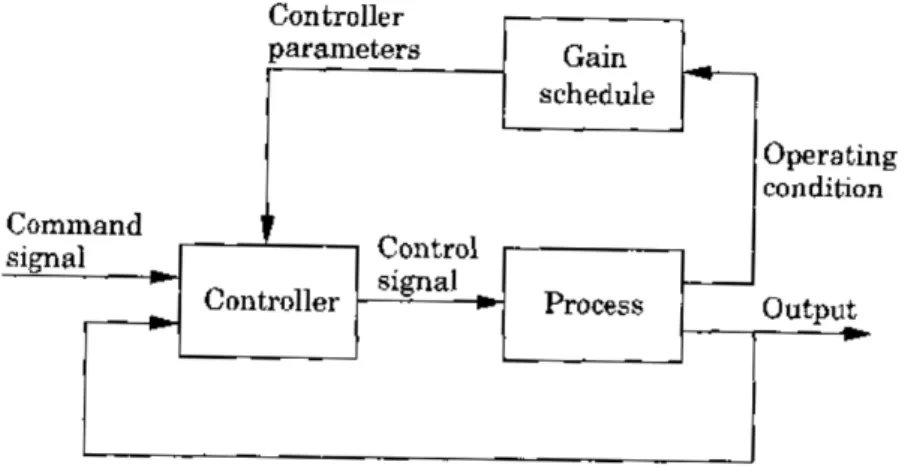
This method is applied when it is possible to find measurable system dynamic’s variables that represent in a trustworthy way the changes in behavior. It is called gain scheduling because originally it was used to measure the gain and then change the controller parameter, that is, schedule them (K. J. Åström & Wittænmark, 1994). Figure 2.16 represents a structure diagram of a gain scheduling controller.

Figure 2.16 - Block diagram of a system with gain scheduling (K. J. Åström & Wittænmark, 1994).

These kinds of controllers are intimately close with the development of flight control systems. In the application mentioned in K. J. Åström & Wittænmark (1994), the two variables were Mach number and altitude, measured by air data sensors.

The gain scheduling is a very suitable technique to reduce the effects of parameter variations (K. J. Åström & Wittænmark, 1994).

2.3.6.2 Model-Reference Adaptive Systems

(49)

23

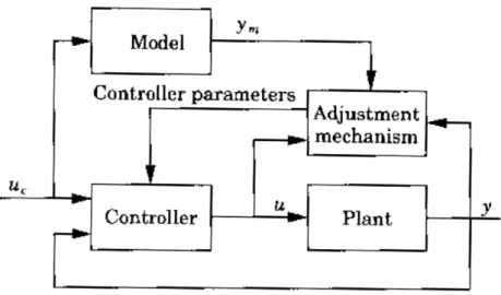
Figure 2.17 - Block diagram of a MRAS (K. J. Åström & Wittænmark, 1994)

The major problem with MRAS is finding the adjustment method in order to obtain a stable system, bringing the error to zero. This is not an insignificant problem. The first MRAS adjustment method was called MIT2_{rule, represented in the next}

equation (K. J. Åström & Wittænmark, 1994):

𝑑𝜃

𝑑𝑡 = −γ𝑒 𝑑𝑒

𝑑𝜃 (2.3.9)

In equation (2.3.9), 𝑒 = 𝑦 − 𝑦𝑚 represents the model error and θ is a controller parameter. The quantity 𝑑𝑒_𝑑𝜃 is the sensitivity derivative of the error and the parameter γ is the adaptation rate. To find the sensitivity derivate approximations are necessary.

The MIT rule can be considered a gradient method to minimize 𝑒2_{(K. J. Åström} & Wittænmark, 1994).

(50)

24

2.3.6.3 Self-tuning Regulators

The adaptive methods supra are known as direct methods because the adjustment rules directly imply the changes in the controller parameters. A different method is encountered if an estimator of how the system parameters are updated is used to adjust the controller parameters (K. J. Åström & Wittænmark, 1994). The block diagram corresponding to this architecture is shown in Figure 2.18 - Block diagram of a STR (K. J. Åström & Wittænmark, 1994).

Figure 2.18 - Block diagram of a STR (K. J. Åström & Wittænmark, 1994).

The controller’s name is meant to underline that the parameters are automatically tuned in order to obtain the closed-loop system proprieties desired. STR are a very flexible scheme, since the controller design and the estimation methods can vary in many ways (K. J. Åström & Wittænmark, 1994).

In STR control method, the process or controller parameters are updated based on real time estimations. These estimations are then used as the real parameters. This is called the certainty equivalence principle. The quality of the estimations can be measured in the same schemes and then used in the controller design. In some cases, the uncertainty is too large and one may choose a conservative method instead (K. J. Åström & Wittænmark, 1994).

(51)

25

2.3.7 Supervised Control

Supervised control is part of the everyday use of an industry. For instance, a human operator adjusting the parameters of a PID controller to account for changes in the environment, is a supervised control. Here, the human operator is a component of the feedback loop adjusting the dynamics using logic-based decisions (J. Hespanha, 2001).

The supervisor functions ensure that the controllers’ action is only applied when the proper excitation is available. Situations like first phase of load disturbance response, bumpless transfer at parameter or controller changes and sometimes dead zones are operating conditions that the algorithms of control are not design for. The supervisor takes these situations into account, in order to maintain the stability and robustness of the systems (Hägglund & Aström, 2000).

The problem is the control of complex systems for traditional methods of control to provide a reasonable performance. There are several ways to improve the performance of a system applying the supervision to control methods, such as: switching control, reconfigurable control and adaptive control.

The main objective of the supervisor is to monitor the signals that can be measured and decide, in real time, whether to apply a different controller or just adapt the controller’s parameters (J. Hespanha, 2001).

In Figure 2.19 the components of a supervisor are embodied. ℙ represents a process, ℂ a controller, 𝔼 an estimator, 𝕄 the monitoring signals and 𝕊 signifies the switching logic (J. Hespanha, 2001).

(52)

26

Supervised control systems tend to appear in real life application where faults are a concern. Because of this, fault detection/diagnosis and fault tolerant control are commonly seen side by side with the supervisor. More on Fault detection/diagnosis and fault tolerant control will be exploited in the next topic.

2.3.8 Fault Detection/Diagnosis and Fault Tolerant Control

In the generic common sense, a failure is something that changes the behavior of a system in a way that it no longer satisfies its purpose. It may be an internal event in the system breaking the power supply, information links or for instance, leakages in pipes (Blanke et al., 2006). Faults are a deviation from the accepted behavior, of a property of a system, they can lead the system to a failure (Cardoso, 2006).

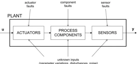
In order to better understand these events, plant faults can be categorized in three groups: actuator faults, component faults (faults in the framework of the process) and sensor faults (Frank, 1996). Figure 2.20 gives a diagram of these categories. The propagation of faults can deteriorate or damage machines and humans; therefore, the quick discovery of faults is imperative in order to stop the propagation of their effects. The controller should be able to measure these fault effects and make the system fault tolerant. In case of success, the system may be able to satisfy its purpose, possibly after a short time of degraded operation (Blanke et al., 2006).

(53)

27

Figure 2.20 - Categories of faults in a system (Brito Palma, 2007).

It is very important to note the distinction of notions between fault and failure. As explained supra, faults cause a change in the characteristics of a component, changing the component performance and operation mode in an undesired way. Still, a fault can be dealt with by a fault tolerant control, keeping the faulty system operational (Cardoso, 2006).

On the other hand, failure is characterized by incapacitating the system or component to fulfill its function. Failure, as it is an irrecoverable event, implies the shutdown of the system. With these notions clear, the idea of fault tolerant control is to prevent a fault from causing a failure at the system level (Blanke et al., 2006).

There are certain requirements and properties which respect systems subjected to faults:

 Safety is a major requirement in order to protect technology from permanent damage as well as humans. The inability to shut-down immediately and guarantee the system to reach a safe status is also a requirement (Blanke et al., 2006).

 Reliability is the probability that a system can fulfill its purpose for a specific period of time, under normal condition. Fault tolerant control have no influence in the reliability of the process components; although it has a major influence in the overall system reliability (Cardoso, 2006).  Availability is the likelihood of a system to be operational when needed.

(54)

28

 Dependability includes all the three properties supra. A dependable system is a fail-safe system with great reliability and availability (Brito Palma, 2007).

Because safety is the most important of all four properties mentioned before, its relation with fault tolerance is now explained in more detail. Assuming that the system’s performance can be described, for instance, by a two dimensional space.

Figure 2.21 shows the two dimensions where the performance regions are delimited. In the region of required performance, the system fulfills its function. This is where the system should be during its operation time. The controller assures that the system remains in this region despite disturbances or model uncertainties used in the controller design

(55)

29

The region of degraded performance demonstrates where the faulty system is allowed to stay. Faults are the reason for the system to go from required performance to degraded performance. Although the performance in this region is not the required, the system can still operate with considerably degraded performance. Fault tolerant controllers should be able to bring the system back from degraded performance into required performance in order to prevent the system from falling into unacceptable or dangerous performance. At the borders the supervision system enters in action, diagnosing the fault and adjusting the controller to the new situation (Blanke et al., 2006).

The region of unacceptable performance should never be reached - it lies between the regions of acceptable performance and the danger zone where the safety of the system is on the line. In order to stay out of the danger zone, the system interrupts its operation avoiding damage to itself and its surroundings. This shows that safety systems and fault tolerant controllers work in separate regions allowing its design without the need to meet safety standards (Blanke et al., 2006).

Before jumping into fault tolerant control architectures, fault types regarding temporal behavior must be defined. They can be defined in additive, multiplicative or intermittent which are represented in Figure 2.22 (Cardoso, 2006).

Figure 2.22 - Fault types regarding temporal behavior (adapted from Cardoso, 2006))

Regarding structures of fault tolerant controllers, there are several possibilities. One example of a fault tolerant control structure is represented in Figure 2.23. There are two major blocks regarding the fault tolerant control:

 Fault diagnosis: where the existence of faults must be detected and identified. This is done by measuring inputs and outputs and testing their consistency with the model (Brito Palma, 2007).

(56)

30

These components cannot be done by an usual feedback controller; instead they need a supervision system (2.3.7 Supervised Control), in order to advocate the control scheme and select the algorithm and/or parameters of the feedback controller (Blanke et al., 2006).

Figure 2.23 - Fault tolerant control architecture (Blanke et al., 2006).

There are three methods used to stablish a fault tolerant control: Reconfigurable Control, Robust Control and Adaptive Control. Adaptive Control and Reconfigurable Control are considered active control technics in response to faults. Differently, Robust Control is a passive method of reacting to faults.

2.3.9 Reconfigurable Control

(57)

31

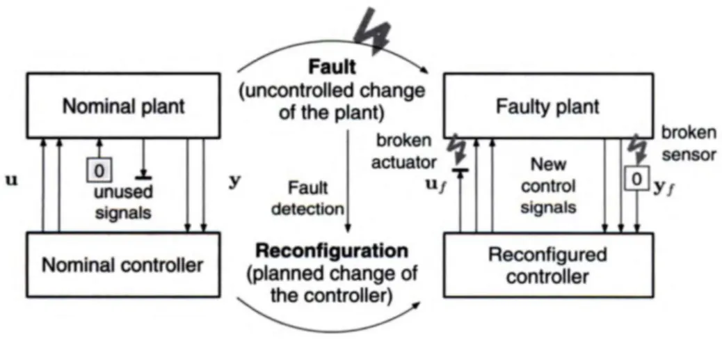
This approach is commonly the second step of fault tolerant control, dealing with the possibility of an important signal path (actuator, sensor, etc.) being broken. In order to restore the control of the system, it is required to find a new solution for the system in order to circumvent the broken link. As the signal path is part of the physical design and construction of the system, it is almost never changeable or repairable right away. However, changes can be made to the control structure of the system (Steffen, 2005). Figure 2.24 shows a diagram of reconfiguration of control reacting to either a broken sensor or an actuator.

Figure 2.24 - Reconfiguration control in response to a fault (Steffen, 2005).

2.3.10 Over-actuated Systems

Recently, much importance has been placed on over-actuated systems. They can provide redundancy for systems, allowing potential recovers from non-nominal conditions. When a system has more actuators than axes to control, it is considered an over-actuated or redundant system. Because of this redundancy, Control Allocation,

(58)

32

2.3.11 Control Allocation

Control allocation algorithms are used in automatic distribution of control in a system. There are several techniques to allocate control such as explicit ganging, pseudo control, pseudo inverse and daisy chaining. As these are the simplest methods, they have disadvantages – neither can guarantee the violation of the rate and position limits of actuators. Some of them are even difficult to apply due to the need to derive a control mixing law a priori. Control allocation algorithms are used in order to compute a unique solution to the problem.

Usually, control allocation algorithms are seen as optimization problems, making all degrees of freedom available to use and, if necessary, allowing secondary objectives to be achieved if needed.(Oppenheimer et al., 2006). There is another control allocator method called direct allocation. This one finds the control vector that results in the best estimation of the command vector (Durham, 1993). The methods mentioned before are well explored in Oppenheimer et al., 2006.

2.3.12 Optimal Control

Optimal control deals with the problem of discovering the control parameters for a certain system, in order to fulfill a certain criteria, usually called cost function. The technique emerged in the 1950s from the work of Lev Pontryagin and Richard Bellman (Bryson, 1996).

An optimal control is composed by a set of differential equations that describe the path of control variables that minimize the cost function. There are many optimization approaches to solve engineering and control problems, such as neural networks and genetic algorithm (Brito Palma, Vieira Coito, Gomes Ferreira, & Sousa Gil, 2015). The Particle Swarm Optimization is amongst them and will be described

infra.

2.3.12.1 Particle Swarm Optimization

(59)

33

Each particle is characterized by their position and speed on a controller’s parameter space being updated according to equation (2.3.10).

𝑝𝑖(𝑛) = 𝑝𝑖(𝑛 − 1) + 𝑠𝑖(𝑛) _(2.3.10)

The position of the particles i at iteration n is 𝑝𝑖(𝑛) and 𝑠𝑖(𝑛) is the speed. The speed is updated according equation (2.3.11).

𝑠𝑖(𝑛) = 𝑤 𝑠𝑖(𝑛 − 1)

+ 𝑐1 𝑟𝑎𝑛𝑑(. ) (𝑜𝑖(𝑛 − 1) − 𝑝𝑖(𝑛 − 1)) + 𝑐2 𝑟𝑎𝑛𝑑(. ) (𝑜𝑔(𝑛 − 1) − 𝑝𝑖(𝑛 − 1))

(2.3.11)

Where w, 𝑐1 and 𝑐2 are real value parameters, 𝑜𝑖(𝑛) is the location of the best position of particle i history, 𝑜𝑔(𝑛) is the location of the best position found by any particle and the random real value vector rand(.) is homogeneously distributed in the range [0; 1]. Each particle position is evaluated using a cost function.

2.4 Related Work

Along the years, there has been some developments in multirotors research area. Up next there are some recent works with some knowledge bases for the research of this thesis.

(60)

34

Figure 2.25 - Samir Bouabdallah’s micro-quadcopter (Bouabdallah, 2007).

In 2008 the Instituto Superior Técnico da Universidade Técnica de Lisboa published a master’s thesis in the quadcopter area. The work was done by Sérgio Eduardo Aurélio Pereira da Costa with the title “Controlo e Simulação de um Quadrirotor convencional”. The work had the objective of modeling, simulating and controlling an unmanned aerial vehicle with rotary thrusters. The design was similar to a quadcopter containing four rotors and a X shaped frame. Pereira da Costa implemented a Kalman filter, in order to observe the global sates of the system, a linear quadratic regulator and a linear Gaussian regulator (Pereira da Costa, 2008). The prototype is in Figure 2.26.

Figure 2.26 –Sérgio Costa’s prototype (Pereira da Costa, 2008).

(61)

35

Figure 2.27 - José Sousa’s Quadcopter (Alves de Sousa, 2011).

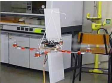
More recently, in 2012, there was a paper published in The International Journal of Robotics Research where the study intent was to design dynamically feasible trajectories and controllers. The paper objective was the development of trajectories and controllers that allow the conventional quadcopter to fly aggressively, maneuvering through narrow spaces, vertical gaps, and land in any angle surface with high precision. The controllers were designed according to a dynamic model and then adjusted in an automated method to the real quadcopter Figure 2.28. Experimental trials took place and are available for watching at https://www.youtube.com/watch?v=MvRTALJp8DM (Mellinger, Michael, & Kumar, 2012).

(62)

36

(63)

37

Chapter 3

3 Modeling, Identification and Control

3.1 Introduction

This section introduces the X8-VB Quadcopter. First, there is a detailed description of the hardware involved in the structure from the power source to the processing unit. Modelling and control are next, where the model techniques and parameters are explored and then control algorithms are developed. Last but not least, fault tolerance control algorithms take place. This chapter follows the diagram already mentioned in 1. Introduction and also presented next in Figure 3.1.

(64)

38

3.2 High Level Architecture

The high level architecture can be seen in Figure 3.2. A specific explanation of each block will be described next. The specifications of each component is presented in order to introduce their main characteristics and the ones that affectthe aircraft directly.

Figure 3.2 - High level hardware architecture.

3.3 Hardware Architecture and Specifications

3.3.1 Frame

The frame was chosen according to the size and material resistance, since the possibility of malfunctions and falls are to be considered, as this is only a prototype where experimental testing will be implemented. DJI Flamewheel 450 was chosen due to resistance and building quality.

(65)

39

The adapter was made out of plastic and contemplates two parts - the upper and lower one, as shown in the Figure 3.3.

Figure 3.3 – 3D model of upper and lower sides of the adapter.

After assembling the eight motors with the propellers, there was the need to build another extension in order to make space for the propeller to rotate freely. With this extension, it was possible to create another level for the battery lowering the center of gravity. The extension is shown in Figure 3.4.

(66)

40

The creations of the complete 3D model (Figure 3.5) then took place in order to implement a virtual simulation. A problem was encountered at this stage. Because the model was too rigorous, Simulink 3D was not able to work with it due to the heavy computational calculations. The solution was to create a simplified model (Figure 3.6) just to represent the process dynamics in the virtual world.

Figure 3.5 - Complete 3D model.

(67)

41

3.3.2 Power Unit

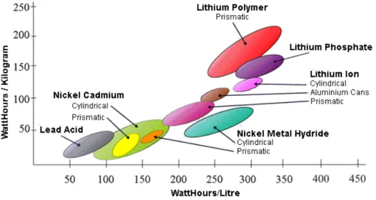
As previously mentioned, LiPo batteries are the most common power supplies among drones. Due to the discharge rate needed to the BLDC motors, the LiPo technology is the best choice. Another very important property of these types of batteries is the power density, demonstrated in Figure 3.7.

Figure 3.7 - Weight and dimension related to power density3_{(Alves de Sousa, 2011).}

Two types of batteries were chosen in this research: the first with 5000 mAh of capacity and 25-35C of discharge rate and the second with 6000 mAh of capacity and 25-50C of discharge rate. The different capacity size and discharge rate were an approach to study the difference of performance and fly time of the multirotor. Both the batteries have 4 Cells with sum to 14.8 V of output voltage. They also have matched impedance. Figure 3.8 shows both selected batteries.

(68)

42

Figure 3.8 - On the left, the 6000 mAh battery. On the right, the 5000 mAh battery.

A very important note is that each cell inside the batteries should never be lower than 3V. In case of voltage lower than 3V, the damage to the battery cells could be destructive or even ignite the battery.

3.3.3 Processing Unit

In order to control the multirotor, there will be two controllers on board. One is the result of the controllers designed in this research and the other one works as a failsafe, in case there is a misplaced controller or a controller fault. The latter is a NAZA Lite V2 from DJI, which will only be activated in case of emergency, applying its control only to the upper motors. This presents the tolerant control even if the controller design in this work fails. The switching command is operated manually with the human interface controller.

The controllers designed will be implemented in one Arduino DUE. This board contains a 32-bit ARM core microcontroller working at 84 Mhz, along with 54 digital input/output pins (of which 12 can be PWM outputs) and 12 analog inputs. A more complete description can be seen in Table 3.1.

Table 3.1 - Arduino DUE specifications (Source: Arduino).

Specification Value

Microcontroller AT91SAM3X8E

Operating Voltage 3,3 V

Input voltage (recommended) 7 – 12 V

Input voltage limits 6 – 16 V

Digital I/O Pins 54 (of which 12 provide PWM output)

(69)

43

Analog Output Pins 2 (DAC)

Total DC Output Current on all I/O lines

130 mA

DC Current for 3.3V Pin 800 mA

DC Current for 5V Pin 800 mA

Flash Memory 512 KB all available for the user applications

SRAM 96 KB (two banks: 64KB and 32KB)

Clock Speed 84 MHz

Length 101.52 mm

Width 53.3 mm

Weight 36 g

3.3.4 Communication Modules

In order to communicate with a base station and with the human controller, there are two communication lines - 433 Mhz radio frequency (RF) and 2.4 Ghz Wi-Fi frequency. The two frequencies were necessary in order to prevent miss communication or interference between commands.

3.3.4.1 RF Communication

The 433 Mhz radios are used to allow the on-board data to reach the base station. The radios are a 2 way full-duplex through adaptive TDM, making it possible to send and receive data simultaneously, with the ability to use “clear to send” and “request to send” signals (see Figure 3.9) The serial communication is made at a 57600 baud rate - in other words, symbols per second or pulses per second.

(70)

44

The connection to the base station are made by USB processed by Matlab . The connections to the Arduino DUE are represented in Figure 3.10, using the serial communication (RX/TX).

Figure 3.10 - Arduino Due and 3DR pin connections.

The 3DR Radio V2 is based on HopeRF’s HM-TRP module as it is equipped with UART interface, transparent serial link, and MAVLink protocol framing. It is also capable of reconfiguring the duty cycle and error correction up to 25% of the bit errors. More detailed specifications are presented in Table 3.2:

Table 3.2 - 3DR Radio V2 specifications.

Max. Output power 100 mW

Receive sensitivity -117 dBm

Operation frequency 433 – 915 mHz

Supply voltage 3.7 – 6 Vdc

Transmit current 100 mA at 30 dBm

Receive current 25 mA

Serial interface 3.3 V UART

(71)

45

3.3.4.2 Human Interface Controller

The controller is composed by two elements: the controller itself and the receiver. The controller is where the human interface is and the receiver is assembled in the aircraft, in order to receive the commands in real time.

The controller chosen was the FrSky Taranis X9D Plus (Figure 3.11). The choice was not only because it runs over an open source system but also because of its exceptional programed communication protocol. The controller provides innumerous buttons in order to interact with the aircraft. One of the buttons is particularly important because it allows the change between control units.

Figure 3.11 – FrSky Taranis X9D Plus on the right and the receiver on the left.

The receiver FrSky X8R (Figure 3.11) has 8 channel outputs and supports telemetry system; therefore, some flight parameters are shown in the controller’s screen in real time. The parameters are: the altitude, the GPS coordinates and the battery voltage. The receiver, beyond the smart port where the sensors are connecter, also supports SBus and RSSI ports.

3.3.5 Sensors

(72)

46

3.3.5.1 GPS

The GPS sensor is the GTOP PA6B and is integrated in a shield that also includes a Micro SD card for data logging. The GPS comes along with an integrated ceramic antenna and a Farad capacitor to replace the external battery for real time clock (RTC) use. Table 3.3 shows some specifications:

Table 3.3 - Shield GPS Logger specifications

Sensibility -165 dBm

Frequency of update 10 Hz

Channels 66

Current consumption 20 mA

The shield can be seen in Figure 3.12.

Figure 3.12 - Shield GPS Logger.

3.3.5.2 Absolute Orientation Sensor

The Absolute Orientation Sensor is a 9 axis motion shield from Bosch. The shield is based on the BNO055 orientation sensor. It has an integrated triaxial 14-bits accelerometer, a triaxial 16-bits gyroscope with ±2000 degrees per second, a triaxial geomagnetic sensor and a 32-bits microcontroller running the BSX3.0 FusionLib software.

The signals provided by the shield are:

Setembro, 2016 Vasco da Silva Brito

Fa u lt To le ra n t Co n tro l o f a X8-VB Qu a d c o p te r

Acknowledgments

Abstract

Resumo

Notations and Symbols

Table of Contents

List of Figures

List of Tables

Chapter 1

1

Introduction

1.1

Motivation

1.2

Main Goals and Contributions

1.3

Thesis structure

Chapter 2

2

State of the Art

2.1

Introduction

2.2

Multirotors

2.2.1

History

2.2.2

DC Motors

2.2.3

Propellers

2.2.4

Energy Power Source

2.3

Control Approaches

2.3.1

PID

2.3.1.1

Proportional Action

2.3.1.2

Integral Action

2.3.1.3

Derivative Action

2.3.2

Fuzzy

2.3.2.1

Membership Function

2.3.2.2

Fuzzification

2.3.2.3

Inference

2.3.2.4

Defuzzification

2.3.3

SMC

2.3.3.1

Sliding Mode Concept

2.3.4

Digital Control

2.3.5

Robust Control

2.3.6

Adaptive Control

2.3.6.1

Gain Scheduling

2.3.6.2

Model-Reference Adaptive Systems

2.3.6.3

Self-tuning Regulators

2.3.7

Supervised Control

2.3.8

Fault Detection/Diagnosis and Fault Tolerant Control

2.3.9

Reconfigurable Control

2.3.10

Over-actuated Systems

2.3.11

Control Allocation

2.3.12