Thermal Analysis of Hollow Tubular Sections under High Temperatures

Thermal Analysis of Hollow Tubular Sections under

High Temperatures

E.M.M. Fonseca

Department of Applied Mechanics, Polytechnic Institute of Bragança, Campus de Sta Apolónia, Apartado 1134, Portugal efonseca@ipb.pt

Abstract- This work presents a numerical model for thermal analysis of steel hollow tubular sections under high temperatures. Curved and straight pipes are structural tubular elements of essential application in the fluids transport, chemical processes or energy generation plants, eventually subjected at mechanical and thermal loading conditions. Hollow tubular sections may have internal voids filled with air (hollow columns, profile sections thermally insulated or steel pipes). The internal temperature should be calculated with some simplified formulas obtained from heat transfer equations. The results obtained in this work, using the internal void formulation, were compared with the thermal response from finite element formulation, for heat conduction with internal insulation and with corresponding results obtained using the simplified heat conduction equation, according Eurocode 3. For small values of the pipe thickness, the thermal behaviour may be determined with high accuracy using one-dimensional mesh approach, with axisymmetric boundary thermal conditions across section.

Keywords- Hollow Tubular Section; Pipe; Internal Void

I. INTRODUCTION

Tubular structures exhibit complex deformations fields given their toroidal geometry, and the multiplicity of the configuration of external loading conditions. Beyond the usual case of these structures subjected to mechanical loads, tubular structures are frequently exposed to aggressive thermal loads. The complexity of this analysis will need some numerical techniques with high performance, which is the case of the finite element analysis here described and studied by different researches [1-3]_{. For steel structures}

design numerous research reports, thesis and scientific papers were published by other authors [4-8]_{. The author of}

this work developed a finite element program to model the thermal behaviour of tubular sections exposed to thermal conditions [5-8]_{. In this work different hollow tubular steel}

sections will be submitted to external fire conditions to verify the temperature level through all components. The hollow tubular sections will be studied considering different boundary conditions, externally radiation and convection due fire conditions, and inside cross-section filled with air or considering internal void. The internal voids temperature will be calculated using a simplified equation. The obtained numerical results will be compared using one and two dimensional finite element solution, and the simplified equation from Eurocode 3 [9]_{. Conclusions are presented and}

discussed about the importance of the temperature field obtained in hollow tubular sections using two and one-dimensional finite element modelling.

II. THERMAL ANALYSIS: HEAT CONDUCTION

The governing equation for transient heat conduction is represented in Equation 1, and as referred by[1-3].

t C Q z z y y x

x ∂

∂ = +      

∂ ∂ ∂

∂ +      

∂ ∂ ∂

∂ +      

∂ ∂ ∂

∂ _λ θ _λ θ _λ θ _{ ρ} θ ₍₁₎

λ

is the thermal conductivity, Q the heat generated by unit volume,

ρ

the material specific mass, C the specific

heat,

θ

the temperature and

t

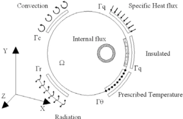
the time.

The temperature field which satisfies Equation (1) in Ω, must satisfy the following boundary conditions: prescribed temperatures θ on a Part Γ_θ of the boundary; specified heat flux

q

on a Part Γ_q of the boundary; heat flux by convection between a Part

Γ

_c of the boundary at Temperature

θ

, heat flux by radiation between a Part Γ_r of the boundary at Temperature

θ

and the environment at the Temperature θ∞, as shown in Figure 1.

Figure 1 Boundary conditions used in heat transfer

The convection global effect is calculated by the following equation on Γ_c:

) ( − _∞ = c θ θ

c h

q (2)

where

h

_c is the heat transfer coefficient by convection. The heat radiation flux through a part Γ_r of the boundary at the Temperature θ and the environment at the absolute Temperature θ_a is represented by Equation (3).

4 4 2 2

( ) ( )( ) ( ) ( )

r

r a a a a r a

h

q =βε θ θ− =βε θ +θ θ θ θ θ+ − =h θ θ−

β is the Stefan-Boltzmann constant,

ε

is the emissivity

and

h

_r is the heat transfer coefficient by radiation. III. THERMAL ANALYSIS: TEMPERATURE INSIDE THE VOID

Using finite elements to discretize the domain, a weak formulation weigh functions based on the Galerkin Method is used, giving rise to a system of differential equations as follows:

F

θ

C

Kθ+  = ₍₄₎

or e h cr h i e q q i e i j m j e j i j m j e h e i i e j i cr e j i j i j i d h N d q N d Q N d N CN d n N N d N N h d z N z N y N y N x N x N e e e e e e Γ + Γ − Ω =         Ω +               Γ ∂ ∂ − Γ + Ω       ∂ ∂ ∂ ∂ + ∂ ∂ ∂ ∂ + ∂ ∂ ∂ ∂ ∞ Γ Γ Ω = _Ω = Ω Γ Γ

∫

∫

∫

∑ ∫

∑ ∫

∫

∫

θ ρ λ λ λ λ θ θ   θ θ 1 1 (5)

m is the total number of elements, N_i and N_j represent

element shape functions.

Based on Equation 5, for the heat transfer and considering the hypothesis: the product between specific heat and air density can be neglected, and air thermal conductivity neglected when compared with steel thermal conductivity, as referred by different researches [10-12]_{; the}

following equation makes possible the temperature development inside the void.

∑ ∫

∑ ∫

= Γ = Γ

Γ

Γ

=

FR e h FR e h N e e h m l N e e h l l Void

d

h

N

N

d

h

N

1 1

θ

θ

(6)

where N_FR is the number of boundary elements at void region, h is the coefficient by convection and corresponds to

the assumption of a non-participating media in the cavity (where air is transparent to radiation) and θ_l is the calculated temperature at each element node. At any time the fictitious temperature inside void will be considered uniform, determined by the heat fluxes received from all the elements surrounding that region.

IV. STEEL THERMAL PROPERTIES

The steel thermal properties as function of temperature as referred in Eurocode 3 [9]_{. The unit mass of steel}

_ρ

_may

be considered a temperature independent parameter and equal to 7850[kg/m3_{]. The specific heat of steel in [J/kgK],}

should be determined from the following equations:

C C C C C C C C C º 1200 º 900 º 900 º 735 º 735 º 600 º 600 º 20 650731 17820 545 738 13002 666 10 22 . 2 10 69 . 1 10 73 . 7

425 1 3 2 6 3

< ≤ < ≤ < ≤ < ≤         − + − + × + × − × + = − − − θ θ θ θ θ θ θ θ θ (7)

The thermal conductivity of steel in [W/mK], should be determined from the following:

C C C C º 1200 º 800 º 800 º 20 3 . 27 10 33 . 3 54 2 < ≤ < ≤     − × = − θ θ θ

λ (8)

V. TEMPERATURE FOR UNPROTECTED INTERNAL STEELWORK

For an equivalent uniform temperature distribution in the cross-section, the increase of temperature ∆θ_a,t in an unprotected steel member during a time interval ∆t is

determined from the simplified equation from Eurocode 3 [9]_.

t h C

V A

k m _netd sh

t

a = ∆

∆ _, /  _,

ρ

θ

(9)

where

k

_sh is the correction factor for the shadow effect,

V

Am/ is the section factor for unprotected steel members [m-1], A_m is the exposed surface area of the member per unit

length [m2/m], V the volume of the member per unit length [m3_/m],

d , net

h the design value of the net heat flux due to convection and radiation per unit area given by expression:

r , net r , n c , net c , n d ,

net h h

h =

γ

 +

γ

 [W/m2] (10)

c n,

γ and

γ

_n,r are factors equals to unity, h_net,c should be calculated according the equation:

, ( )

net c c m

h =h θ_∞−θ [W/m2] (11)

c

h

should be taken as 25[W/m2K],

θ

m is the surface temperature of the member,

θ

_∞ is the gas temperature of the surrounding environment member in fire exposure, given in Equation 12.

A standard temperature-time curve ISO 834 was adopted which is given by the following equation, according Eurocode 1 [13]:

10 20 345log (8 1)t

θ_∞= + + (12) t is the time in minutes [min].

r , net

h is the design value of the heat flux due to radiation

per unit area given by expression:

] ) 273 ( ) 273 [( 10 67 .

5 8 4 4

, =Φ⋅ ⋅ × ⋅ + − +

− m r res r net

h ε θ θ [W/m2] (13)

Φ

is the configuration factor, which should be taken equal unity,

θ

r is the radiation temperature of the environment of the member usually taken as

θ

_r=

θ

∞,

∆

t

time interval, which should not be taken as more than 5 seconds and

ε

_res is the resultant emissivity.

VI. STUDY CASE

shown in this figure and the thermal properties considered, according Eurocode 3 [9]_{. Four different hollow tubular}

sections were studied with the following relations between thickness and section medium radius hr: 0.235, 0.118, 0.02

and 0.007, where medium radius is equal to 170[mm] and thickness was considered equal to 40, 20, 3.4 and 1.2[mm], respectively. Using the finite element program, three different simulations were considered for each other: considering an internal void (using Equation 5), an insulated internal region and an internal cavity filled with air (considering a solid internal mesh with thermal air properties). For external boundary conditions, fire conditions were assumed. According to the Eurocode 1 [13]_,

in structural surfaces exposed to fire conditions, the convection coefficient is equal to 25[W/m2_{K] and the}

emissivity equal to 0.5. For regions not exposed to fire, in this case, inside the cross-section, the convection coefficient is equal to 9[W/m2_{K] and the radiation effect is neglected.}

These conditions will be applied for inside void in all tubular sections.

Figure 2 The Biot number

A. Lumped Capacitance Method Application

The thermal transient analysis can be performed by applying the so-called lumped capacitance method [14, 15]_.

This method requires the temperatures gradients within the solid to be negligible. The Biot number permits measuring how well this condition is approximated. The Biot number is a dimensionless heat transfer coefficient and is defined as the ratio between the thermal resistance to convection and the thermal resistance to conduction, as the following equation:

λ

c c i

h

L

B

=

(14)

where

L

_c is the characteristic length of the solid,

defined as a ratio between the volume and the surface area of the solid,

λ

is the thermal conductivity of the solid and

c

h

is the convection coefficient with air.

Figure 2 shows the Biot number for all studied cases using the Equation 14 and the thermal conductivity depending on temperature.

In all studied cases the Biot number is below 0.078. When Bi<<1, it is considered a uniform temperature through the cross solid section at any time during the transient heat process [15]_{. Based on the assumption of a}

spatially uniform temperature distribution inside the solid throughout the transient process the lumped capacitance method could be applied. The temperature of a solid as a function of time could be calculated using the Equation 15.

(

)

( )

∞ ⋅ −

∞

+

−

=

θ

θ

θ

θ

BiFo

i

t)

e

( (15)

where

θ

_(t)

−

θ

_∞ is the temperature difference at time

t

,

∞

−

θ

θ

_i is the temperature difference at time

t

=

0

and

Fo

is the Fourier number.

The dimensionless Fourier number is calculated for a time after step-change in ambient temperature, function of the thermal conductivity, density and specific heat of solid body, according the following equation:

2

c

L

C

t

Fo

ρ

λ

=

(16) The results obtained from lumped capacitance method will be presented and compared with the numerical results and the simplified equation from Eurocode 3 [9]_.

VII. RESULTS AND DISCUSSION

The temperature field was obtained using two and one-dimensional finite element meshes. For a two-one-dimensional mesh, only one-quarter of section was considered, as show in Figure 3b in radial tubular direction. Due to the symmetry of boundary condition and geometry, only an angular segment would be used. For one-dimensional mesh the entire pipe length in longitudinal direction was used, Figure 3c.

a)

b) c)

Figures 4, 5 and 6 represent the temperature field obtained in a thick tubular section (h/r=0.235) using a two-dimensional mesh.

Figure 4 Temperature field obtained with internal insulated region

Figure 5 Temperature field obtained with an internal modelled air

Figure 6 Temperature field obtained with internal void

The results were obtained by finite element formulation and compared with the solution obtained using the simplified equation from Eurocode 3 [9]. Changing the relation, the temperature across the pipe thickness varies and the simplified equation does not correspond to the actual value. The same is applied for the one-dimensional mesh. It is possible to conclude, the one-dimensional modelling may be applied to thin tubular sections, giving good results. Figures 7 to 10 show the temperature evolution for all studied hollow tubular sections, using the finite element

solver for two and one-dimensional meshes. The results are compared with the simplified equation from Eurocode 3 [9]

for all different section factors and with lumped capacitance method using Equation 15.

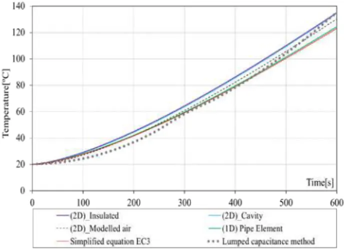
Figure 7 Time history of temperature, hr=0.235

Figure 8 Time history of temperature, h r=0.118

Figure 10 Time history of temperature, hr=0.007

For thin structural pipes, the temperature variation across thickness is small and does not increase with fire action. For higher tubular thickness, the curves are not coincident, with a temperature variation, as can be seen using the two-dimensional models. The calculated Biot number, smaller than 1, determines uniform temperature fields inside the body. The temperature evolution calculated from lumped capacitance method agrees well with all results presented.

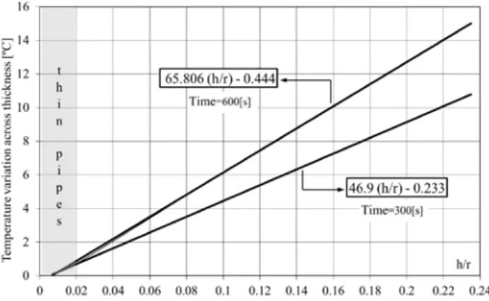
Figure 11 represents the temperature variation across tubular thickness for different relations hr at two different

instant times.

Figure 11 Temperature variation across pipe thickness

In tubular sections due to the axisymmetry, considering the same boundary conditions along the section radius, the inside surface temperature is uniform. As temperature is uniform inside voids, heat flux by radiation should not be considered, neglecting this type of heat transfer in tubular structures. Decrease of temperature gradient across the pipe thickness has been verified for thin structures and a uniform temperature should be considered as well the Eurocode 3 proposals [9]_{, with the simplified heat equation. It is possible}

to obtain the temperature field for thin tubular structures using one-dimensional finite element model.

VIII. CONCLUSIONS

The obtained results permit comparing different calculations, including one and two dimensional finite

element solution, and the simplified equation from Eurocode 3 [9]_{. The two dimensional solutions were applied}

for the case of thick tubular structures. For thin-walled tubular section, a simplified one dimensional solution as well as the Eurocode 3 simplified equation [9] is acceptable and should be applied. According to results from Figure 10, thick tubular structures should be considered for grater values than h/r=0.02.

The modelling of internal voids is important during the temperature evolution in structural elements. The computing effort on meshing the internal void (filled with air) will be greater than the simplified formula used to model the internal void, with no advantage in temperature calculation. The results obtained with the developed program have been compared with the simplified heat conduction equation proposed by Eurocode 3 [9]_{. Based in the analysed case}

study, it is concluded that for thin tubular structures (h/r<0.02), the temperature field can be obtained with less computational effort using one-dimensional mesh for an external axisymmetric boundary condition. With this condition, the internal temperature of the pipe is uniform because there is no heat exchange by radiation in the cavity. We can neglect what happens in the internal void, except if there is a forced longitudinal ventilation of cold air or an induced fluid motion.

NOTATION

The following symbols are used in this paper:

V

Am/ = section factor for unprotected steel; m

A

= exposed surface member area per unit length;

i

B = Biot number; C = specific heat;

h = section thickness;

h

_c = heat transfer coefficient by convection; cr

h

= combined convection and radiation heat transfer coefficient;

h

r = heat transfer coefficient by radiation; d

net

h _, = heat flux design value due convection and radiation per unit area;

r , net

h = heat flux design value due radiation per unit area;

sh

k

= correction factor;

c

L = characteristic length;

i

N, N_j =shape functions;

q = specified heat flux; r

q

= heat radiation flux;

Q = heat generated by unit volume;

r

= section medium radius;

t

= time;

V = member volume per unit length;

β = Stefan-Boltzmann constant;

ε

= emissivity; m

f

ε

= emissivity related to the fire compartment;

res

ε = resultant emissivity;

Fo = Fourier number;

θ = temperature;

θ = prescribed temperature;

θ

Void = temperature inside void;

θ

_∞ = environment temperature in member exposure to fire;

λ

= thermal conductivity;

ρ

= material specific mass;

t , a θ

∆ = temperature increase in an unprotected steel member

t

∆ = time interval;

Φ = configuration factor; Ω = domain of heat conduction.

REFERENCES

[1] R. W. Lewis, K. Morgan, H. R. Thomas, K. N. Seetharamu,

The finite element method in heat transfer analysis, John Wiley & Sons, Inc., 1996.

[2] G. Comini, S. Giudice, C. Nonino, Finite element analysis in heat transfer, Taylor & Francis, 1994.

[3] H. C. Huang, A. S. Usmani, Finite element analysis for heat transfer, Springer-Verlag, London, 1994.

[4] J. M. Franssen, R. Zaharia, Design of steel structures subjected to fire, Les Éditions de l’Université de Liège,

Belgique, 2005.

[5] E. M. M. Fonseca, F. J. M. Q. Melo, C. A. M. Oliveira, “The thermal and mechanical behaviour of structural steel piping systems”, International Journal of Pressure Vessels and Piping 2005; vol. 82(2): pp.145-153.

[6] E. Fonseca, P. M. M. Vila Real, “Finite element modelling of thermo-elastoplastic behaviour of hot-rolled steel profiles submitted to fire”, In: R. Abascal, J. Domínguez y G. Bugeda (Eds.), IV Congresso de Métodos Numéricos en Ingeniería, SEMNI - Sociedad Española de Métodos Numéricos en Ingeniería 1999; Spain, ISBN:84-89925-45-3.

[7] E. M. M. Fonseca, F. Q. Melo, R. A. F. Valente, “The flexibility of steel hollow tubular sections subjected to thermal and mechanical loads”, WIT Press Transactions on The Built Environment, M. Guarascio, C.A. Brebbia, F.Garcia,

(Ed.), Second International Conference on Safety and Security Engineering 2007; Malta, ISBN 978-1-84564-068-2, 94: 171-180.

[8] E. M. M. Fonseca, F. J. M. Q. Melo and L. R. Madureira; “Chapter 4: A finite element formulation for piping structures based on thin shell displacements theory”, In: Toroidal Shells, Mechanical Engineering Theory and Applications, Ed. Nova Science Publishers, Inc. New York, Editor: Bohua Sun, ISBN: 978-1-61942-247-6, pp. 115-149, 2012.

[9] CEN, EN 1993-1-2, Eurocode 3: Design of steel structures - Part1.2: General Rules - Structural Fire Design. 2005. [10]J. M. Franssen, Elements of theory for SAFIR 2001 free, A

computer program for analysis of structures submitted to the fire. University of Liege, Belgium, 2002.

[11]J. Palsson, U. Wickström, “A scheme for verification of computer codes for calculating temperatures in fire exposed structures”, In: J.M. Franssen (Ed), Structures in fire - Proceedings of the first international workshop 2000; Copenhagen, 135-148.

[12]E. M. M. Fonseca, C. A. M. Oliveira, “Numerical modelling of internal voids in fire exposed structures”, In: José O. Valderrama, Carlos J. Rojas, (Eds.), 5º Interamerican Congress on Computers Applied to the Process Industry 2001; Brasil, ISBN: 956-291-077-6, 195-199.

[13] BS EN 1991-1-2:2002, Eurocode 1, Actions on structures – Part1-2: General actions–Actions on structures exposed to fire. 2002.

[14] F. P. Incropera, D. P. De Witt, “Fundamentals of heat and mass transfer”, 5th editon, Wiley, NY.

[15] S. Baglio, S. Castorina, L. Fortuna, N. Savalli, “Modeling and design of novel photo-thermo-mechanical microactuators”, Sensors and Actuators,

vol.A101, pp.185-193, 2002.