Lat. Am. j. solids struct. vol.14 número11

Abstract

This work presents a detailed description of the formulation and implementation of the Atomistic Finite Element Method AFEM, exemplified in the analysis of one- and two-dimensional atomic domains governed by the Lennard Jones interatomic potential. The methodology to synthesize element stiffness matrices and load vectors, the potential energy modification of the atomistic finite elements (AFE) to account for boundary edge effects, the inclusion of boundary conditions is carefully described. The conceptual rela-tion between the cut-off radius of interatomic potentials and the number of nodes in the AFE is addressed and exemplified for the 1D case. For the 1D case elements with 3, 5 and 7 nodes were ad-dressed. The AFEM has been used to describe the mechanical behavior of one-dimensional atomic arrays as well as two-dimensional lattices of atoms. The examples also included the anal-ysis of pristine domains, as well as domains with missing atoms, defects, or vacancies. Results are compared with classical molecular dynamic simulations (MD) performed using a commercial package. The results have been very encouraging in terms of accuracy and in the computational effort necessary to execute both methodologies, AFEM and MD. The methodology can be expanded to model any domain described by an interatomic energy potential.

Keywords

AFEM, Interatomic potentials, Lennard Jones potential, molecular dynamics.

Mechanical Behavior of Nano Structures Using

Atomic-Scale Finite Element Method (AFEM)

1 INTRODUCTION

The last decades have witnessed an enormous increase in the development of nanotechnologies, which have brought a large impact on areas such as engineering, medicine, biology, chemistry, as well as in aerospace, construction and manufacturing industries. The scientific community has been

D.A. Damasceno a, * E. Mesquita b

R.N.K.D. Rajapakse c

a

Department of Computational Mechanics, School of Mechanical Engineering, University of Campinas, Mendeleyev, 200, Cidade Universitária, Campinas , SP, 13083-860, Brazil.

Author email: daniela@fem.unicamp.br b

Department of Computational Mechanics, School of Mechanical Engineering, University of Campinas, , Mendeleyev, 200, Cidade Universitária, Campinas , SP, 13083-860, Brazil.

Author email: euclides@fem.unicamp.br

c _{School of Engineering Science. Simon}

Fraser University. 8888 University Drive Burnaby, Canada V5A 1S6

Author email: rajapakse@sfu.ca

* Corresponding author

http://dx.doi.org/10.1590/1679-78254050

working to analyze and develop mechanical, electronic and optoelectronic devices at nano-scale, which can be applied to many areas which range from sensors engineering to medical therapies and drug delivery systems (The Royal Society and The Royal Academy of Engineering, 2004; Novoselov et al., 2012; Chen et al., 2013). Nanomechanics of materials is a new branch of mechanics which studies the properties and behavior of nanoscale materials and structures in response to applied loads and prescribed boundary conditions. From the dimensional perspective, a structure with at least one dimension smaller than 100 nm is considered to be a nanostructure (The Royal Society and The Royal Academy of Engineering, 2004).

The mechanical behaviour of nanoscale systems can be analyzed by using Ab-initio methods (Dirac, 1981), semi-empirical quantum methods (Tadmor and Miller, 2011) and also modified clas-sical continuum mechanics. Ab-initio calculations are most accurate compared to semi-empirical quantum methods, but computationally very expensive and the analyses are still limited to a few hundred or thousand atoms. The molecular dynamics (MD) (Alder et al., 1959) has been one of the most commonly method used to analyze the behaviour of nanomaterials. Although MD methods can be applied to analyze larger systems, than those that can be treated by Ab-initio methods, it is still not applicable to systems consisting of many millions of atoms, which are frequently necessary to model practical devices.

For nanostructures greater than a few nanometres, multi-scale continuum methods such as Gur-tin-Murdoch theory (GM-T) (Gurtin and Murdoch, 1975), that bridges surface and bulk energies, is quite accurate and computationally inexpensive (Dingerville et al., 2005; Miller et al., 2000; Liu et al., 2010; Sapsathiarn et al., 2012). However, GM-T and other continuum methods are not strictly applicable to model discrete atomic structures. The computational cost in modelling nanomaterials is a fundamental challenge. In order to overcome this challenge, the Atomic-scale Finite Element Method (AFEM) was developed and applied for multiscale analysis of carbon nanotubes (CNTs) by Liu and his co-authors (Liu et al., 2004; Liu et al., 2005). Presently, the AFEM can model and ana-lyze the mechanical behavior of many materials at the nanoscale (Malakouti, 2006; Tao et al., 2016; Damasceno et al., 2015).

The AFEM is based on an energy approach. It requires an interatomic energy potential, de-scribing local or non-local bonding forces of an atom interacting with a chosen set of other sur-rounding atoms. The choice of the interacting sursur-rounding atoms and their array will, ultimately, lead to the formulation of the specific Atomic Finite Element. In principle, the method can be ap-plied to all atomic systems that may be described by an interatomic energy potential.

2 ATOMIC SCALE FINITE ELEMENT METHOD FORMULATION

The AFEM, as described by Liu et al. (2004), is based on an energy approach. It requires an intera-tomic energy potential, U, describing local or non-local bonding forces of an atom interacting with a chosen set of other surrounding atoms. The interatomic energy potentials are described in terms of the coordinates of the individual atoms, xi, and some constitutive parameters of the considered atomic elements and arrays.

For a system with N atoms, the total interatomic energy considers the contribution of all inter-acting atoms:

(

)

N

j i

tot i < j

U =

å

U_ij x - x ₍₁₎

Consider the energy W_f, related to the sum of the work of external forces, F_iext acting on indi-vidual atoms indicated by ‘i':

N ext

f i i

i = 1

W =

å

F x (2)

The total energy in this system with N atoms, E_tot, is composed of the interatomic bonding en-ergy and the (eventual) work of external forces.

(

)

N N

ext

j i i

tot i

i < j i = 1

E =

å

U_ij x - x -

å

F x ₍₃₎

As usual, the desired equilibrium condition is obtained by determining the stationary value of the total energy in the system with respect to the position x_i of the individual atoms:

tot

dE = 0

dx (4)

The total energy E_tot can be expanded in a Taylor series around the equilibrium position of the atoms, x( )0 :

( )

( )

( )

( )

( )

(

)

(

( )

)

( )

( )

(

)

0 0

2 T

0 _tot 0 0 _tot 0

tot tot

x = x x = x

dE 1 d E

E x E x + x - x + x - x x - x

dx 2 dxdx

» ₍₅₎

Defining the displacement u as the difference between the actual, x, and the equilibrium posi-tion, x( )0

( )

(

0

)

u = x - x ₍₆₎

( ) { } { }

K u u = P

é ù

ë û (7)

Where é_ëK u

( )

ù_û corresponds to the nonlinear stiffness matrix,

{ }

u , the displacement increment vector and

{ }

P the non-equilibrium load vector, respectively, given by:

( )

( )0 ( )0

2 2

tot tot

x = x x = x

d E d U

K u = =

dxdx dxdx

é ù é ù

ê ú ê ú

é ù _{ê ú ê ú}

ë û _{ê ú ê ú}

ë û ë û

(8)

And

{ }

( )0 ( )0

tot tot

x = x x = x

dE dU

P = - = F -

dx dx

ì ü ì ü

ï ï ï ï

ï ï ï ï

ï ï ï ï

í ý í ý

ï ï ï ï

ï ï ï ï

ï ï ï ï

î þ î þ (9)

3 LENNARD JONES POTENTIAL

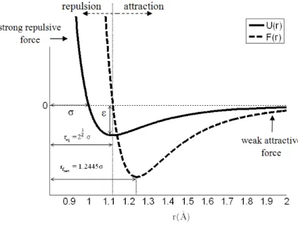
In this section, a brief review of the Lennard-Jones (LJ) potential proposed by Jones (1924) is in-troduced. It is used to calculate the potential energy of the interaction between two non-bonding atoms based on their distance of separation, r_ij:

(10)

Where

(

)

2

(

)

2

ij i j i j

r = x - x + y - y is the bond length, and the r_c is some prescribed cut-off ra-dius, which switches off the atomic interaction when the bond length exceeds its value. Only two Lennard-Jones parameters are sufficient to describe the intermolecular interactions, σ and ε_LJ, as shown in Figure 1. The parameter εLJ is the depth of the potential well and σ is the inter-particle

distance at which the potential is zero. The

12 ij r s æ _ö÷ ç _÷ ç _÷ ç _÷

çè ø term represents the strong repulsion and the

high energy on the bond, as the distance between the pair of atoms decreases. The 6 ij r s æ _ö÷ ç _÷ ç _÷ ç ÷

çè ø term

represents the attractive term, which describes the weak attraction on the bond, as the distance between the pair of atoms increase.

The internal force, F r

( )

_ij , between the two atoms is obtained by differentiating the potential with respect to the intermolecular distance, r_ij:

( )

( )

ij ε σ12 σ6

ij _{13 7}

ij ij ij

dU r

F r = - = 4 12 - 6

dr LJ r r

é ù

ê ú

ê ú

ê ú

ë û (11)

( )

ε σ σ

12 6

ij c

ij ij ij

ij c

4 - for r < r

U r = r r

0 for r r

LJ

ì é ù

ï æ ö æ ö

ï êç ÷ ç ÷ ú

ï êç ÷ ç ÷ ú

ï _ç ÷ _ç ÷

ï _êç ÷_{÷ ç} ÷_{÷ ú}

í _êè ø è ø _ú

ï _{ë û}

ïï _³

Figure 1 shows the LJ potential, U(r), and the interatomic force, F(r), as a function of the

dis-tance, r_ij. By setting the force F r =0

( )

, the equilibrium distance between the atoms, r_eq is found to be:

σ σ

1 6 eq

r = 2 = 1.1225 (12)

If the distance between two atoms is less than r_eq, the Lennard-Jones force is repulsive. If the distance is greater than r_eq, the force is attractive. The maximal force is obtained at the intermo-lecular distance,

σ σ

fmax 6

1

r = = 1.2445

7 26

(13)

It should be noted that for intermolecular distances larger than r_fmax the interatomic bonding force decreases continuously. When the distance between atoms reaches the equilibrium distance

between the atoms, , the bonding force is assumed to vanish.

Figure 1: Lennard-Jones potential U(r), and internal force F(r).

The cut-off radius r_c is an important parameter to be chosen. It determines with how many

neighboring atoms, a given atom is interacting. The cut-off radius r_c also determines whether the atomic interaction has a local or non-local character. In this article the cut-off radius of the intera-tomic bonding will be related to the number of nodes within a specific Aintera-tomic Finite Element. This will be illustrated in the next paragraphs within the context of 1D elements.

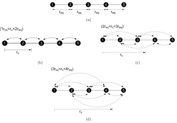
eq

Consider an atomic chain with 5 atoms in equilibrium position, as shown in Figure 2a. Every considered atom interacts with one or more of its neighbors, according to the relation between the interatomic equilibrium distance r_eq and the chosen cut-off radius r_c. Three distinct conditions will be analyzed. First, consider that the cut-off radius obeys the relation (r_eq< r_c < 2r_eq). This means that one atom only interacts with the first nearest neighboring atoms, as shown in Figure 2b. For the second condition, (2r_eq < r_c < 3r_eq), every atom interacts with the first and the second nearest neighboring atoms, as shown in Figure 2c. The third condition, (3r_eq < r_c < 4r_eq), is illustrated in Figure 2d.

Two aspects should be stressed. First, when the cut-off radius is smaller than two times the equilibrium distance, r_c<2r_eq, the atomic bondings have a local character. For larger cut-off radius,

c

r >2r_eq, the bonding extends to the second or more distant neighbors and gives a non-local charac-ter to the incharac-teratomic incharac-teractions. The second comment is related to the finitude of the atomic chain considered. The atoms 1 and 5, indicated in Figure 2a, represent the physical limit of the considered chain. The lack of atoms to the left of atom number 1 and to the right of atom number 5 impacts directly the energy bonds of the chain. If r_c>2r_eq, non-local bonds exist and not only the bond energy of the most external atoms (1 and 5, at the present case) if affected. This must be carefully considered when modelling a bounded atomic domain with the AFEM.

(a)

(b) (c)

(d)

4 ATOMIC FINTE ELEMENTS

In this section the formulation for 1D and 2D Atomic Finite Elements are, exemplarily, presented for the case the Lennard-Jones interatomic potential. The idea is to focus on the fundamental issues of the AFEM formulation and not on material properties of the domains to be analyzed.

4.1 The 1D Atomic Element

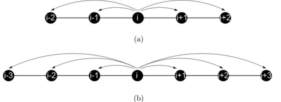
The notion of the atomic finite element will be introduced based on three examples. Consider

Figure 3, showing an atomic finite element with three nodes, designated as i-1, i and i+1. The defi-nition of the atomic finite element and all the derived calculations, such as internal forces and stiff-ness matrix, are related to the central node, in this case, node i. It is assumed that the relation be-tween the equilibrium distance and the potential cut-off radius satisfies (r_eq < r_c < 2r_eq). The arrows in Figure 3 a shows that the central atom i, is only connected to its first neighbor atom to the left (i-1) and to the right (i+1). The total bonding energy for this 3 node atomic finite element i is composed of the bonding (i-1, i) and (i, i+1):

i

tot i,i-1 i,i+1

U = U + U (14)

Figure 3: A three-node atomic-scale finite element.

The expressions for element stiffness matrix, 3e i

K and non-equilibrium force vector, P_i3e and for this atomic three node finite element are obtained by substituting the expression for the bonding energy (14) and the external forces in equations (8) and (9), resulting delivering, respectively:

2 tot

i-1 i

2 2 2

tot tot tot

3e i

i-1 i i i i+1 i

2 tot

i+1 i 3x3

d U 1

0 0

2 d x d x

d U d U d U

1 1

K =

2 d x d x d x d x 2 d x d x

d U 1

0 0

2 d x d x

é ù ê ú ê ú ê ú ê ú ê ú ê ú ê ú ê ú ê ú ê ú ê ú ë û (15) tot 3e ext i i i 3x1 0 d U P = F -

The Lennard-Jones potential is a pairwise potential, describing the interaction between two at-oms, that is the interaction of atom (i) over atom (i+1) and the reciprocal interaction of atom (i+1) on atom (i). In the present formulation the atomic element is represented by node (i) and only the interaction of node (i) with (i-1) and (i) with (i+1) will be considered. This is implied by the direc-tions of the arrows in Figure 3. The reciprocal interaction, of the neighboring atomic element cen-tered in the node (i-1) on the node (i), of the present element, will be added later at the mesh as-sembly procedure. So only half of the bonding energy between (i) and (i-1), and (i) and (i+1) has to be considered. This is expressed by the 1/2 factor in the element stiffness matrix.

Figure 4a shows a 5-node atomic finite element. The central node is denoted by (i) and it inter-acts with the two nearest nodes, (i-1) and (i-2) to the left and (i+1) and (i+2) to the right. For this element the condition (2r_eq < r_c < 3r_eq) is considered. Analogously, for the 7-node element, shown in Figure 4b, the relation between equilibrium distance and cut-off radius is (3r_eq < r_c < 4r_eq).

(a)

(b)

Figure 4: (a) A five-node atomic-scale finite element, (b) a seven-node atomic-scale finite element.

The total bonding energy of these elements are, respectively, given by:

i-5e

tot i,i-1 i,i-2 i,i+1 i,i+2

U = U + U + U + U (17)

i-7e

tot i,i-1 i,i-2 i,i-3 i,i+1 i,i+2 i,i+3

U = U + U + U + U + U + U (18)

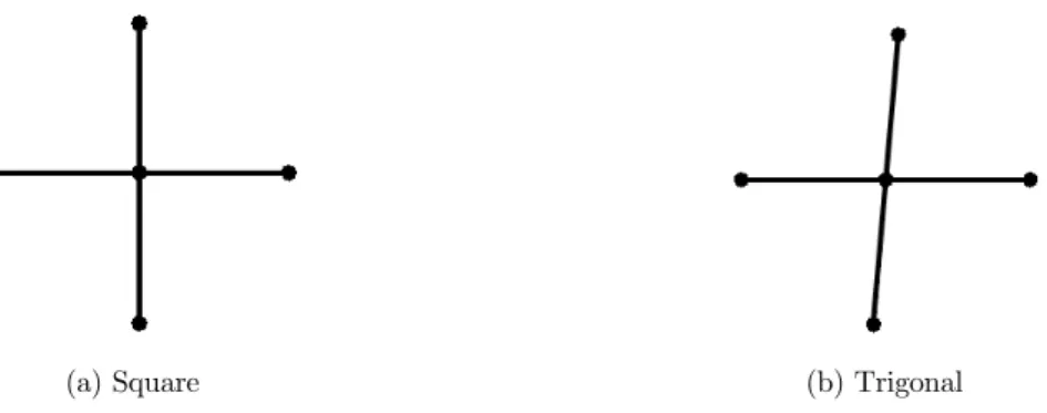
4.2 Atomic Element in Two Dimensions

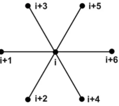
In this section two-dimensional atomic finite elements are presented. The starting point is the 7-node 2D element shown in Figure 5. As it will be shown, it may be used to model the geometry of hexagonal Bravais type lattices (Liu et al., 2006). The central atom, (i), has connection with all of surrounding atoms, (i+1), (i+2), (i+3), (i+4), (i+5) and (i+6). The total energy for this basic 2D 7-node atomic finite element is the sum of all pairwise interacting nodes:

2D_tot

i i,i+1 i,i+2 i,i+3 i,i+4 i,i+5 i,i+6

Figure 5: Atomic finite element with seven nodes.

The element stiffness matrix and the element non-equilibrium force vector for the atomic finite element with seven nodes are given by, respectively:

( ) ( ) ( ) ( ) ( ) ( ) ( ) ( ) ( ) ( ) 2 2 tot tot i i i+3 i+3 2 2 tot tot i i i+3 i+3

2 2 2 2 2 2

tot tot tot tot tot tot

i i i i i i i i

i+3 i+3 i+6 i+6

2

e 2 2

tot tot

i

i+3 i+3

d U d U

0 0 0 0

dx dx dy dx d U d U dx dy dy dy

0 0 0 0

d U d U d U d U d U d U dx dx dy dx dx dx dy dx dx dx dy dx K

d U d U dx dy dy dy

D é _{ù =} ê ú ë û               ( ) ( ) ( ) ( ) ( ) ( )

2 2 2 2

tot tot tot tot

i i i i i i+6 i i+6 i

2 2 tot tot i i i+6 i+6 2 2 tot tot i i i+6 i+6

d U d U d U d U dx dy dy dy dx dy dy dy

0 0 0 0

d U d U dx dx dy dx

d U d U

0 0 0 0

dx dy dy dy

é ù ê ú ê ú ê ú ê ú ê ú ê ú ê ú ê ú ê ú ê ú ê ú ê ú ê ú ê ú ê ú ê ú ê ú ê ú ê ú ê ú ê ú ê ú ê ú ê ú ê ú ê ú ê ú ê ú ê ú ê ú ê ú ë û               (20)

( )

( )

6x1 tot ext i i e tot ext i i 6x1 0 dU F - dx P =

dU F - dy 0 é ù ê ú ê ú ê ú ê ú ê ú ê ú ê ú ê ú ê ú ê ú ê ú ë û (21)

(a) Square (b) Trigonal

Figure 6: Atomic finite elements for different two-dimensional Bravais lattices.

a) Square b) Trigonal

Figure 7: Square and Trigonal f two-dimensional Bravais lattices.

5 AFEM IMPLEMENTATION

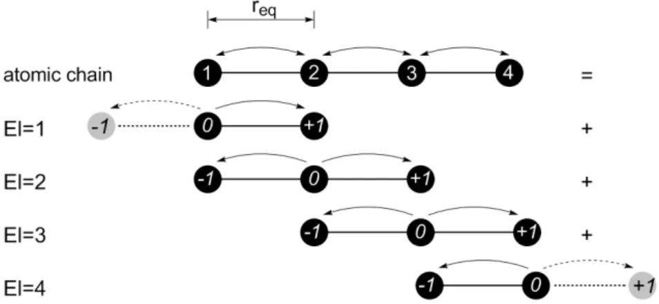
The assemblage procedure in one and two dimensions, the concept of modified atomic finite element and the application of boundary conditions will be discussed in this section. Figure 8 illustrates the AFEM assemblage procedure for a 1D atomic chain containing 4 atoms. The atomic finite element with three nodes is considered. The atomic chain is bounded so that to the left side of atom 1 and to the right side of atom 4 there are no atoms. Because of this lack of neighboring atoms, the atom-ic finite elements on the edges of the mesh must be modified. So even before the imposition of the boundary conditions, the potential energy of the edge element must be modified to account for the non-existence of one or more neighboring atoms.

calculation procedure. Again, the dashed arrow in EI=4, between node (0) and node (+1) illustrates the required modification.

Figure 8: Example of assemblage scheme for an atomic chain of 4 atoms.

The expression for the total energy of the 4 atom chain, Utotal, is given by the sum of the con-tributions of the energy of individual elements, _UEl_{, as shown in equation (22):}

(

El=1 El=2 El=3 El=4

)

total

1

U = U +U +U +U

2 (22)

The the expressions for the energy of each of the 4 atomic elements used to model the 4-atom chain of Figure 8 are given in the expressions (23) to (26):

σ σ

ε

12 6

El=1

12 12

U = 4

-r r

LJ

é_{æ ö æ ö} ù

êç_ç ÷_÷ ç_ç ÷_÷ ú

ê_çç ÷_{÷ çç} ÷_÷ ú

êè ø è ø ú

ë û

(23)

σ σ σ σ

ε ε

12 6 12 6

El=2

21 21 23 23

U = 4 - +4

-r r r r

LJ

é_{æ ö æ ö} ù é_{æ ö æ ö} ù

ê_çç _÷÷ _çç ÷_÷ ú ê_çç _÷÷ ç_{ç ÷}÷ ú

ê_{çç ÷}÷ _çç ÷_÷ ú ê_{çç ÷}÷ _{çç ÷}÷ ú

êè ø è ø ú êè ø è ø ú

ë û ë û

(24)

σ σ σ σ

ε ε

12 6 12 6

El=3

32 32 34 34

U = 4 - +4

-r r r r

LJ

é_{æ ö æ ö} ù é_{æ ö æ ö} ù

ê_çç _÷÷ _çç ÷_÷ ú ê_çç _÷÷ ç_{ç ÷}÷ ú

ê_{çç ÷}÷ _çç ÷_÷ ú ê_{çç ÷}÷ _{çç ÷}÷ ú

êè ø è ø ú êè ø è ø ú

ë û ë û

(25) σ σ ε 12 6 El=4 43 43

U = 4

-r r

LJ

é_{æ ö æ ö} ù

êç_ç ÷_÷ ç_ç ÷_÷ ú

ê_çç ÷_{÷ çç} ÷_÷ ú

êè ø è ø ú

ë û

(26)

The third important stage of the assemblage produce in AFEM is the application of the bound-ary conditions. Figure 9 illustrates the same atomic chain of Figure 8 but including a set of bounda-ry conditions. In this case, the displacement of atom 1 is blocked, so, the degree of freedom of this atom must be excluded from the global stiffness matrix, and from of the global non-equilibrium force vector.

Figure 9: Introduction the boundary conditions at the 4 atoms chain.

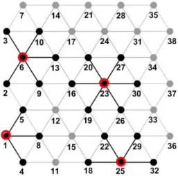
The assemblage procedure of AFEM in two dimensions system is the same used for the one di-mensional system. Figure 10 illustrates an example, which consists of a triangular (hexagonal) mesh with 38 atoms. The basic atomic finite element considered has 7 nodes, and was shown in Figure 5. In order to apply boundary conditions or to analyze meshes with defects and missing atoms, the basic atomic elements must also be modified to account for the missing neighboring atoms. This is illustrated in Figure 10. Element number 23 is an example of a complete atomic element. Elements 1, 6 and 25 are incomplete, or modified elements. Just like the 1D case, the bond energy of the missing neighboring atoms must be excluded from the total energy of the element.

Figure 10: Atomic structure with complete and modified elements.

The total energy expression for the mentioned elements 23, 1, 6, and 25 are:

23

tot 23,16 23,19 23,20 23,26 23,27 23,30

U = U + U + U + U + U + U (27)

1

tot 1,4 1,5 1,8

6

tot 6,2 6,3 6,9 6,10 6,13

U = U + U + U + U + U (29)

25

tot 25,18 25,22 25,29 25,32

U = U + U + U + U (30)

The total bond energy of the complete element 23 and of the modified elements 1, 6 and 25 is given in Table 1. The element energy determined within the atomistic finite element procedure and the corresponding energy obtained by the Molecular Dynamics (MD) package LAMMPS (Plimpton, 1995) are also indicated. It can be seen that the energy for each AFE is distinct, according to the number of missing surrounding atoms. Table 1 also shows that the energy values calculated by AFEM and MD are in accordance.

Total Energy

23 tot

U

_(eV) 1

tot

U

_(eV) 6

tot

U

_(eV) 25

tot

U

_(eV)

AFEM -3.0 -1.50 -2.50 -2.0

MD -3.0 -1.50 -2.50 -2.0

Table 1: Comparison of total element energy obtained from AFEM and MD.

The matrices and load vectors for the complete or modified elements are assembled and, in the sequence, the boundary conditions are imposed. It is stressed again, that modifying the atomic ele-ments to account for missing bonds and the imposition of boundary conditions are two distinct solution steps within the AFEM. In the present implementation the resulting non-linear system, equation (7) was solved iteratively by the Newton-Raphson method.

6 RESULTS

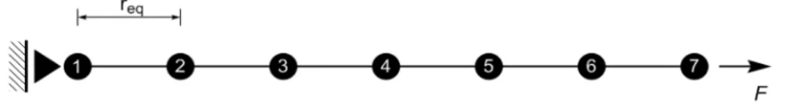
6.1 Comparison of AFEM and MD in One Dimension

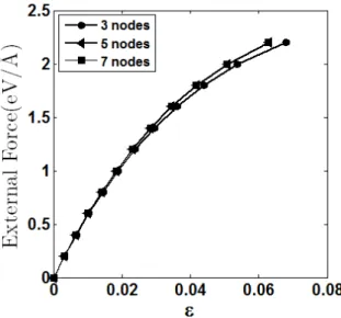
In this section, the 1D AFEM is investigated. Initially, the influence of the number of element nodes in the atomic elements is addressed. As already discussed, the number of nodes in the AFE is related to the chosen cut-off radius for the Lennard Jones potential. The first example is shown in Figure 11. It consists of a 7 atom chain, fixed at atom 1 and loaded by a force F at node 7. This example will be solve using atomic elements with 3, 5 and 7 nodes. Before imposing the boundary conditions, the distance between the atoms is set to be equal to the equilibrium position, r_eq= 1.122 Å. After applying the boundary conditions, the load vector is increased until the atomic chain fails by bond breaking. At every load step the non-linear equation (7) is solved iteratively.

Figure 12 shows the resulting force-strain relations. The strain measure  is obtained by divid-ing the displacement of atom 7, u₇ by the original chain length Lo, = u₇/Lo. The curves show that there is very little difference between the results obtained considering the atomic elements with 5-nodes and 7-5-nodes. It suggests that 1D AFEM simulations using atomic finite element with 5 5-nodes is almost as accurate as atomic finite element with 7-nodes.

Figure 12: External force by strain (3, 5 and 7 nodes elements).

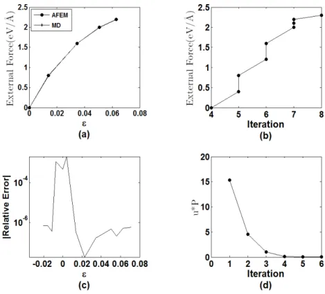
In the sequence, the accuracy of the obtained AFEM results will be validated by comparison with the results obtained from MD package LAMMPS. To simplify, the values of parameters of the LJ potential were assigned unit values, _σ = 1 and _εLJ =1. The AFEM results were determined for the 5 node element. In the MD simulations, the Lennard Jones potential was used at a temperature of 1 K. Non-periodic boundary conditions were used. For the AFEM and MD simulations the cut-off radius is set equal to r_c =2.5s (Smit, 1992). The time integration step for the MD simulations is 0.05 fs.

Figure 13a shows force-strain curves obtained by both methodologies. Figure 13c depicts the relative error between strains obtained by both solutions. There is a good agreement between both solutions, with a relative error smaller that 10-5, except at the initial equilibrium position. The MD simulation needed 1000 iterations to achieve the equilibrium position for every load step. On the other hand, the number of iterations for the AFEM to reach a non-equilibrium force vector smaller than 10-11 for distinct values of the load force is shown in Figure 13b. The number of iterative steps for every force in the AFEM varied from 4 to 8 according to the loading stage.

Figure 13: 1D AFEM results - a) force-strain relation; b) number of iterations for AFEM, c) MD-AFEM relative error, d) convergence measure.

The results of Figures 13a to 13d suggest that the 1D AFEM formulation and implementation is correct, that the results are accurate and the number of iterative steps, required for the solution, is significant smaller than those of the typical MD simulations.

6.2 Comparison of AFEM and MD in Two Dimensions

This section is dedicated to the study of a 2D AFE. A two-dimensional hexagonal (or triangular) lattice, shown in Figure 14, presenting 655 atoms is analyzed. The 2D atomic finite element (AFE) with 7 nodes, given in Figure 5, is considered. Zero displacement boundary conditions are imposed on all atoms on the left edge, shown inside of the red dashed box. External force with the same amplitude are applied on all atoms on the right edge in x direction, as shown by the arrows in Fig-ure 14. The Lennard Jones potential was used in MD at a temperatFig-ure of 1 K. The Lennard-Jones potential parameters are, s =1= and e_LJ =1. The cut-off radius for the MD simulations is set to

c

r =1.5Å. Non-periodic boundary conditions were used.

Figure 15a shows a force-strain diagram obtained by AFEM and MD. The results are obtained for the central atom at the left border of the mesh. A similar result, showing the change in total

length of the atomic mesh, L, is given if Figure 15b. The AFEM and MD solutions agree very

50000 iterative steps to achieve a final configuration with 4 significant digits, whereas the AFEM never needed more than 7 steps to achieve the same accuracy.

Figure 14: A schematic diagram of a two-dimensional lattice.

As a second 2D example, consider the same mesh of the previous example, shown in Figure 16. Zero displacement boundary condition imposed to the atoms within the red dashed box at the left border. An external force Fext is applied in the vertical direction upon atom number 739. The black lattice in Figure 16 represents the original atomic mesh. The blue mesh shows the deformed mesh at its last loading step before bond breaking. The atom 739 is connected to atoms 728 and 729 as illustrated in the detail shown in Figure 16. It is simple to see that the bonding force between atoms 739 and 729 is in compression and that the force between atoms 739 and 728 is traction.

Figure 17 shows in dashed lines the interatomic bonding force developed by the Lennard-Jones potential as a function of the interatomic distance r_ij, as anticipated by equation (11). This figure also show the bonding forces between atoms 739-729 (compression) and between atoms 739-728 (traction) for distinct amplitude stages of the external force, Fext. Traction is marked in blue color and compression in red color.

As expected, the interatomic bonding forces start with a zero value at the equilibrium position and increase continuously in traction and compression for increasing values of the external load. The bonding forces follow exactly the path predicted in equation (11). It should be noticed that this is a highly non-linear behavior, in which interatomic displacements for compressed bonds is much smaller than those of the traction bonds for the same external loading level. Figure 17 also shows the break bonding situation. After the condition, in which the traction bond, in blue, reaches the maximum bonding force at r_fmax = 1.2445 σ, given by equation (13), the bonding forces decrease for larger distances, the bond can no longer withstand the imposed external loads and breaks. The iterative system will no longer converge, unless a new mesh without the lose atom is considered.

Figure 17: internal force by r.

In the third example, the effect of missing atoms or vacancies on the mechanical behavior of an atomic mesh is investigated. Figure 18a shows a pristine mesh, with no vacancies. On the other hand, Figure 18b depicts the same mesh but with 4 missing atoms. In both cases, zero displacement boundary conditions are prescribed for the atoms in the right edge within the red dashed box. A force of equal, increasing amplitude is applied to the 4 atoms at the left border. The external load is increased incrementally until one or more atomic bonds within the mesh break. Figure 18c shows the stress (force)-strain behavior of the pristine and of the defect mesh. The same strain measure of the previous examples is used. It can be seen that vacancies do have a large effect on the force-strain behavior. For validation purposes, Figure 18d depicts the deformed configuration of the de-fect mesh (Figure 16b), determined by AFEM and MD. There is a good visual agreement between the two methodologies.

(a) (b)

(c) (d)

Figure 18: (a) Pristine mesh; (b) Defected mesh, (c) stress-strain curves, and (d) final equilibrium configuration from AFEM and MD.

(a) (b)

Figure 19: (a) Square bravais lattice; (b) Force-strain curves obtained from AFEM and MD.

0 0.02 0.04 0.06 0.08

0 10 20 30 40 50 60 70



Str

e

s

s

(G

P

a

)

7 CONCLUSIONS

This work presents a detailed description of the formulation and implementation of the Atomistic Finite Element Method (AFEM), exemplified in the analysis of one- and two-dimensional atomic domains governed by the Lennard-Jones interatomic potential. The methodology to synthesize ele-ment stiffness matrices and load vectors, the potential energy modification of the atomistic finite elements (AFE) to account for boundary edge effects, the inclusion of boundary conditions were carefully described, in a way that the authors had not previously found in the AFEM literature. The conceptual relation between the cut-off radius of interatomic potentials and the number of nodes in the AFE is addressed and exemplified for the 1D case. For the 1D case elements with 3, 5 and 7 nodes were addressed. The AFEM has been used to describe the mechanical behavior or one-dimensional atomic arrays as well as two-one-dimensional lattices of atoms. The reported studies also included the analysis of pristine domains, as well as domains with missing atoms, defects, or vacan-cies. Almost all results were compared with classical molecular dynamic simulations (MD) per-formed using a commercial package. The results have been very encouraging in terms of accuracy and in the computational effort necessary to execute both methodologies, AFEM and MD. The methodology presented can be extended to other potential, like Tersoff (Tersoff, 1987), REBO (Brenner, 1990), AIREBO (Stuart, 2000), which have been applied to model nano structures com-posed of graphene and materials alike.

Acknowledgments

The research leading to this article has been funded by the São Paulo Research Foundation (Fapesp) through grants 2012/17948-4, 2013/23085-1, 2015/00209-2 and 2013/08293-7 (CEPID). Support from CAPES and CNPQ has been fundamental to the development of the present re-search. This is gratefully acknowledged.

References

Alder, B.J., Wainwright, T.E.J. (1959). Studies in Molecular Dynamics. I. General Method, The Journal of Chemical Physics 31: 459-466.

Brenner, D.W. (1990), Empirical potential for hydrocarbons for use in simulating the chemical vapor deposition of diamond films, Physical Review B 42: 9458.

Chen, C., Hone, J. (2013). Graphene Nanoelectromechanical Systems. Proceedings of the IEEE 101(7).

Damasceno, D.A., Rajapakse, R.K.N.D., Mesquita, E. (2015). Mechanical behavior of atoms using atomic-scale finite element method. Proceedings of the XXXVI Ibero-Latin American Congress on Computational Methods in Engineer-ing.

Dingerville, R., Qu, J., Cherakoui, M. (2005). Surface free energy and its effect on the elastic behavior of nano-sized particles wires and films, Journal of the Mechanics and Physics of Solids 53: 1827-1854.

Dirac, P.A.M. (1981). The Principles of Quantum Mechanics, Clarendon Press, Oxford.

Gurtin, M., Ian Murdoch, A. (1975). A continuum theory of elastic material surfaces, Archive for Rational Mechan-ics and Analysis 57: 291-323.

Kim, K. (2006). The Atomic-scale Finite Element Method for Analyzing Mechanical Behavior of Carbon Nanotube and Quartz, M.Sc. Dissertation, Virginia Polytechnic Institute, Virginia.

Liu, B., Huang, Y., Jiang, H., Qu, S., Hwang, K.C. (2004). The atomic-scale finite element method, Computer Meth-ods in Applied Mechanics and Engineering 193: 1849-1864.

Liu, B., Jiang, H., Huang, Y., Qu, S., Yu, M.F. (2005). Atomic-scale finite element method in multiscale computa-tion with applicacomputa-tions to carbon nanotubes, Physical Review B, 72: 1098-0121.

Liu, C., Rajapakse, R.K.N.D. (2010). Continuum models incorporating surface energy for static and dynamic re-sponse of nanoscale beams, IEEE Transactions on Nanotechnology 9: 422-431.

Liu, W.K., Karpov, E.G., Park, H.S. (2006). Nano Mechanics and Materials: Theory, Multiscale Methods and Appli-cations, John Wiley & Sons.

Malakouti, M., Montazeri, A. (2016). Nanomechanics analysis of perfect and defected graphene sheets via a novel atomicscale finite element method, Superlattices and Microstructures 94: 1 -12.

Miller, R.E., (2000). Size-dependent elastic properties of nanosized structural elements, Nanotechnology, 11:139-147. Nanoscience and nanotechnologies: opportunities and uncertainties (2004). The Royal Society and The Royal Acad-emy of Engineering, London.

Novoselov, K.S., Fal′Ko, V.I., Colombo, L., Gellert, P.R., Schwab, M.G., Kim, K. (2012). A roadmap for graphene, Nature 490: 192.

Plimpton, S. (1995), Fast Parallel Algorithms for Short-Range Molecular Dynamics, Journal of Computational Phys-ics 117: 1-19.

Sapsathiarn, Y., Rajapakse, R.K.N.D. (2012). A model for large deflections of nanobeams and experimental compari-son, IEEE Transactions on Nanotechnology 11, 247-254.

Smit, B. (1992), Phase diagrams of Lennard-Jones fluids, The Journal of Chemical Physics 96: 8639-8640.

Stuart, S.J.; Tutein, A.B.; Harrison, J.A. (2000), A reactive potential for hydrocarbons with intermolecular interac-tions, The Journal of Chemical Physics 112: 6472 -6486.

Tadmor, E.B., Miller, R.E. (2011). Modeling materials: continuum, atomistic, and multiscale techniques. Cambridge University Press, New York.

Tao, J., Sun, Y., (2016). The Elastic Property of Bulk Silicon Nanomaterials through an Atomic Simulation Method. Journal of Nanomaterials 2016: 6.