DOI: http://dx.doi.org/10.1590/1806-9126-RBEF-2018-0035 Licença Creative Commons
Comparing the Schrödinger and Dirac Descriptions of an
Electron in a Uniform Magnetic Field
David Velasco Villamizar
∗1, Benjamin Russell
21Departamento de Física, Universidade Federal de Santa Catarina, CEP 88040-900, Florianópolis, SC, Brasil 2Princeton University, Departament of Chemistry, Frick Laboratory, Princeton, New Jersey, United States of America
Received on February 5, 2018; Revised on April 15, 2018; Accepted on April 20, 2018.
In this article we present a detailed description, using ladder operators, of an electron in a uniform magnetic field evolving under the Schrödinger equation. We go on to describe the same physical system in terms of relativistic quantum mechanics using the Dirac equation and to compare the two models in detail. The main differences between these two quantum mechanical approaches are discussed and we observe specifically how the relativistic phenomena modify the description of this particular quantum system by isolating effects which only exist in the relativistic model.
Keywords:Quantum Mechanics, Schrödinger Equation, Dirac Equation, Uniform Magnetic Field
1. Introduction
In this article we present the detailed calculations re-quired for a didactic comparison between the dynamics of the Schrödinger and Dirac equations for an electron in a uniform magnetic field. This is done in order to juxtapose these two quantum mechanical descriptions of the same system as a pedagogic tool. This comparison is not found in any quantum mechanics textbook known to the authors. For this reason, our analysis provides an invaluable resource to instructors, who could make use of this example, either for an advanced undergraduate quantum mechanics course or for a beginning graduate course.
It is well known that one of the simplest phenomena at the quantum scale is the interaction between an elec-tron (a spin one half fermion) and an external uniform axial magnetic field [1–6]. Although this physical system comprises only a single particle, whether it is at rest or in motion, its description is valuable as it furnishes the many of basic concepts required to understand other more complex phenomena. For specific examples see both elec-tron vortex beams [7–9] and the interaction of solid state materials with magnetism [10–14] (known as the integer Quantum Hall effect). Additionally, this specific physical system shows a certain isomorphism to quantum optics, demonstrating a narrow relation to describe the Gaus-sian beam profile of electromagnetic radiation, leading to orthogonal states known as Orbital Angular Momentum of light [15]. The relevant optical phenomenon have been studied experimentally due to the high accuracy now achievable and the wide applicability [16] of simulations
∗Endereço de correspondência: [email protected].
in innumerable quantum systems of interest. For example, the orbital angular momentum Hall effect [17], which is an analogue to the integer quantum Hall effect.
A brief outline of this paper follows. In section 2 we describe the interaction between spin1/2 and a uniform magnetic field. In section 3 we describe in detail the Schrödinger equation of the electron in motion under the interaction of the external magnetic field, performing the analysis by using the ladder operator method. Con-sequently, we can notice that the wave function of the electron exhibits a cylindrical symmetry, this feature is related to the uniform nature of the external magnetic field. We explain briefly the equivalence between the electron eigenstates and the Laguerre-Gaussian modes, which are characteristic of the orbital angular momen-tum of light in cylindrical coordinates. We then further present a short discussion about the electron energy lev-els and the Landau levlev-els. Finally, in section 4 we present a relativistic analysis using the Dirac equation for the electron wave function and discuss the main differences to the Schrödinger equation description.
2. Spin-magnetic field interaction
Here we consider the quantum description of an electron initially at rest in a uniform external magnetic field. We consider the electron magnetic dipole moment ~µ=
−me
0
~
ˆ
S, where (e= 1,6021×10⁻¹⁹C) is the modulus of the fundamental electric charge and the vectorial spin operatorS~ˆ=~
simplify the calculations we assume the orientation of the magnetic field is along the zˆaxis, accordingly the electrons Hamiltonian is given by,
ˆ
H = e~B 2m0
1 0
0 −1
. (1)
The energy levels are E± =±~ω/2, where ω = eBm0 is
the precession frequency of the magnetic dipole moment around the external field, known as Larmor Frequency. In addition, the eigenstate of positive energy is|0i=1
0
and the negative energy is |1i=0 1
. These eigenstate are related to the spin orientation when aligned or anti-aligned to the magnetic field, respectively.
3. Schrödinger equation of an electron in
magnetic field
In contrast to the previous section, here we present a quantum description of an electron in motion in a region with a uniform external magnetic fieldB~. In the classical
description, the electron follows a helical path along the magnetic field showing an axial symmetry. Accordingly, we apply a gauge transformation to the magnetic vector potential to take into account this symmetry. In particu-lar, the specific symmetric gauge transformation is well known as the Landau gauge,
~ A(~r) = 1
2 B~ ×~r
. (2)
The linear momentum operator ispˆ→pˆ−q ~A, where the
electron charge is given by q=−e. Then, in terms of
momentum, the Hamiltonian is,
ˆ
H= 1 2m0
ˆ
p+e ~A2+ e
m0
~ B·S,~
= −~ 2
2m0∇
2+e2A2 2m0−
ie~ 2m0 ∇·
~
A+A~·∇+ e
m0
~ B·S.~
(3)
The second term of the Hamiltonian can be expanded,
e2A2 2m0
= e 2
8m0
~ B×~r2,
= e 2
8m0B
2r2sin2(θ Br),
= e 2
8m0
B2r2−(B~·~r)2,
(4)
whereθBr is the angle between the magnetic field and
the electron vector position. The third term in Eq. (3) can be calculated using,
∇· Aφ~ = ∇·A~φ+A~·∇φ. (5)
The first term in the last expression is equal to:
∇·A~φ= 1
2∇· B~ ×~r
φ,
= 1
2 ∇ ×B~
·~rφ−1
2 ∇ ×~r
·Bφ,~
= 0.
(6)
This shows that the Landau gauge satisfies the Coulomb gauge. Continuing the calculation of the second term in Eq. (5) in a similar way,
~
A· ∇φ= 1 2 B~ ×~r
·∇φ,
= 1
2B~· ~r× ∇
φ.
(7)
Representing the differential operator in terms of the quantum linear momentum operator it follows that,
~
A· ∇φ= i
2~B~· ~r×Pˆ
φ,
= i 2~B~·Lφ.ˆ
(8)
Eliminatingφfrom the above results allows us to write
the Hamiltonian (3) as,
ˆ
H=−~ 2
2m0∇ 2+ e2
8m0
B2r2−(B~·~r)2+ e 2m0
~
B·Lˆ+2 ˆS. (9)
For simplicity and without loss of generality, we are going to assume a uniform magnetic field aligned alongzˆaxis. Consequently, the Hamiltonian can now be written,
ˆ
H = −~ 2
2m0∇
2+e2B2 8m0
x2+y2+ eB 2m0
ˆ
Lz+ 2 ˆSz,
= −~ 2
2m0
∂2
∂z2 +
−~2 2m0
∂2
∂x2 +
∂2
∂y2
+e 2B2 8m0
x2+y2+ eB 2m0
ˆ
Lz+ 2 ˆSz.
(10) According to this result, one notices the contributions of various terms of different respective natures. These are, a free particle alongzˆaxis, a two-dimensional harmonic oscillator in x−y plane with its projection of angular
momentum alongzˆaxis and, finally, the electron spin in-teraction with the magnetic field. We can expressψ(~r, σ), the associated electron wave function, as the product of functions in according with these features,
ψ(~r, σ) =F(x, y)eipzz/~Γ, (11) where the spinorial function is,
Γ =
1
0
, ms= +1/2
0 1
, ms=−1/2 , (12)
andms is the quantum number equal to the spin
projec-tion along the magnetic field direcprojec-tion.
We can analyze the two-dimensional harmonic move-ment of the electron to obtain the Schrödinger equation for a quantum harmonic oscillator,
−~2 2m0
∂2
∂x2+
∂2
∂y2
+1 2m0ω
2x2+y2
| {z }
H′
xy
whereω= eB
2m0 is the harmonic frequency. The quantum
harmonic oscillator is,
E′ =~ω(nx+ny+ 1),
=~ω(n+ 1), n≥0. (14)
We note that each energy levelE′
n, is related to (n+ 1)
degenerate eigenstates Fnx,ny,
Fn,0, Fn−1,1, · · · , F0,n. (15)
In relation to this degeneracy, we look for a physical quantity which enables a better characterization of states belonging to a certain energy level. Given the spatial symmetry of the harmonic potential under a rotation around thezˆaxis and the axial component of the orbital angular momentum of the electronLˆz= ˆxpˆy−yˆpˆx, we can analyze the two-dimensional motion of the electron by applying the ladder operator method to each Cartesian coordinate,
ˆ
ax= 1
√
2 xβˆ +i ˆ
Px
β~ !
, aˆ†x= 1
√
2 xβˆ −i ˆ
Px
β~ !
,
ˆ
ay = 1
√
2 yβˆ +i ˆ
Py
β~ !
, ˆa†y= 1
√
2 yβˆ −i ˆ
Py
β~ !
,
(16)
where the constantβ=pm0ω
~ is reciprocal to the natural length of the harmonic oscillator [2]. Moreover, these operators satisfy the following commutation relations [ˆax,ˆa†x] = [ˆay,ˆa†y] = 1. Furthermore, we can expressxˆ,yˆ,
ˆ
px,pˆy, as a function of the ladder operators. Accordingly,
we have,
ˆ
x= 1
β√2 ˆax+ ˆa
†
x
, Pˆx=−i ~β √
2 ˆax−aˆ
†
x
,
ˆ
y= 1
β√2 ˆay+ ˆa
†
y
, Pˆy =−i ~β √
2 ˆay−ˆa
†
y
.
(17)
The angular momentum operator is given by, ˆ
Lz=i~ ˆaxˆa†y−ˆa†xˆay
. (18)
Similarly, we can express the harmonic Hamiltonian as,
ˆ
H′
xy=~ω ˆa†xˆax+ ˆa†yaˆy+ 1. (19)
Calculating the commutation relation between the angu-lar momentum and the Hamiltonian yields:
ˆ
Hxy′ ,Lˆz
=
~ω ˆa†xˆax+ˆa†yˆay+1, i~ˆaxˆa†y−ˆa†xaˆy
,
=i~2ω −aˆxˆa†y+ˆa†xaˆy+ˆa†yˆax−ˆayˆa†x), = 0.
(20)
Thus, we can show thatLˆz is a constant of motion. Con-sequently, the angular momentum operator has the same
set of eigenstates as Hˆ′
xy; in this way, we can expose
an axial symmetry in the system. As such, we are go-ing to implement the cylindrical coordinate system to describe the quantum operators corresponding to the electron position and momentum. Additionally, we will borrow from geometrical optics the notion of the Jones’ vectors for the circular polarization of light [18]. One can introduce new ladder operators related to the axial symmetryaˆR andˆaL, which are right and left circular
operators respectively. These are denoted as a function of the Cartesian ladder operators as,
ˆ
aR= 1
√
2 aˆx−iaˆy
, ˆaL= 1
√
2 ˆax+iˆay
. (21)
Particularly, when these operatorsˆaRandˆaL act on the
eigenstateFnx,ny, they generate a quantum state which is a linear combination ofFnx−1,ny andFnx,ny−1. This results in a state with energy smaller by~ω.
Contrast-ingly,ˆa†R andˆa†L generate a quantum state with energy
larger by~ω.
Moreover, these operators satisfy the following com-mutation relations,
ˆ
aR,ˆa†R
=ˆaL,ˆa†L
= 1. (22)
Hence, we can express,
ˆ
a†RˆaR= 1 2 aˆ
†
xˆax+ ˆa†yˆay+i(ˆaxaˆ†y−ˆa†xˆay)
,
ˆ
a†LˆaL= 1 2 aˆ
†
xˆax+ ˆa†yˆay−i(ˆaxaˆ†y−ˆa†xˆay)
.
(23)
This leads us to express Hˆ′
xy andLˆz as, ˆ
Hxy′ =~ω NˆR+ ˆNL+ 1, Lˆz=~ NˆR−NˆL, (24)
whereNˆR= ˆa†
RaˆR andNˆL= ˆa†LaˆL are known as the
Her-mitian number operators. When acting on the eigenstate
Fnx,ny, these operators simply evaluate to a positive in-tegernRandnL, respectively. The physical meaning of
these numbers is related to the current energy level, as we will show later.
We denote the ground state (the state of lowest energy) byF0,0. In relation to this state, we can express any other eigenstate as a consecutive action of the operators ˆa†R
andˆa†L,
FnR,nL= 1 p
(nR)!(nL)!
(ˆa†R)nR(ˆa† L)
nLF
0,0. (25)
SinceFnR,nL is a set of eigenstates in common toHˆ
′
xy
andLˆz, we can obtain the energy levels~ω(n+1)and the
corresponding eigenvaluesml~. In this way, we can define
the main quantum numbernand the orbital quantum
numbermlas a function ofnR andnL,
SincenRandnL are positive integers, there are (n+1)
degenerate eigenstates for every energy level, as shown in Eq. (15). This proves the next relation,
nR=n ; nL= 0
nR=n−1 ; nL= 1,
...
nR= 0 ; nL=n.
(27)
Considering the particular casen= 0,1and its possible values ofml, we have,
n= 0 ⇒ nR= 0, nL= 0 → ml= 0
n= 1 ⇒
nR= 1, nL= 0 → ml= +1
nR= 0, nL= 1 → ml=−1 .
(28)
In general, for every fixed value of n, there is a set of
values ofml,
ml=n , n−2, n−4, · · · , −n+ 2, −n. (29)
By virtue of this change of notation, we can express the eigenstateFnR,nL by using the pair of quantum numbers
n, ml, which are a more appropriate characterization
of this quantum system arising from the observableLˆz. Thus, we have,
F
nR=n+ml
2 , nL=
n−ml
2
. (30)
Then, we use the cylindrical coordinates,
x=̺cosϕ y=̺sinϕ z=z
, ̺≥0, 0≤ϕ <2π, (31)
We can rewrite the Hamiltonian of the two-dimensional harmonic oscillator in this coordinate system. The set of operatorsˆaR andˆaL transform as,
ˆ
aR=√1
2 ˆax−iaˆy
,
=1 2
ˆ
xβ+iPx β~
−i
ˆ
yβ+iPy β~
,
=1 2
β xˆ−iyˆ+ i
~β Pˆx−iPˆy
,
=1 2
β x−iy+1
β
∂ ∂x−i
∂ ∂y
.
(32)
The radial distance and the azimuthal angle are defined as̺=px2+y2andϕ=arctan(y/x). We can verify that,
x−iy=̺ cosϕ−isinϕ=̺e−iϕ, (33)
and the Cartesian differentiation will be written as,
∂ ∂x =
∂̺ ∂x
∂ ∂̺+
∂ϕ ∂x
∂
∂ϕ = cosϕ ∂ ∂̺−
1
̺sinϕ ∂ ∂ϕ, ∂
∂y = ∂̺ ∂y
∂ ∂̺ +
∂ϕ ∂y
∂
∂ϕ= sinϕ ∂ ∂̺ +
1
̺cosϕ ∂ ∂ϕ,
(34)
Then,
∂ ∂x−i
∂ ∂y
= cosϕ−isinϕ ∂ ∂̺
−1
̺ sinϕ+icosϕ
∂
∂ϕ,
=e−iϕ
∂ ∂̺ −
i ̺
∂ ∂ϕ
.
(35)
Thus, the operatorsaˆRandˆa†R can be expressed in
cylin-drical coordinate as,
ˆ
aR=
e−iϕ 2
β̺+ 1
β ∂ ∂̺−
i β̺
∂ ∂ϕ
,
ˆ
a†R=e iϕ
2
β̺−β1∂̺∂ −β̺i ∂ϕ∂
.
(36)
Analogously, we can obtain,
ˆ
aL=
eiϕ 2
β̺+ 1
β ∂ ∂̺+
i β̺
∂ ∂ϕ
,
ˆ
a†L= e
−iϕ
2
β̺−β1∂̺∂ + i
β̺ ∂ ∂ϕ
.
(37)
In particular, the action ofˆaRorˆaL on the ground state
FnR=0,nL=0 is,
ˆ
aRF0,0=e
−iϕ
2
β̺+1
β ∂ ∂̺ −
i β̺
∂ ∂ϕ
F0,0, = 0.
(38)
This result means physically the impossibility of annihi-lating a quantum of energy~ωfrom the ground state. In
virtue of this fact, we can solve the differential equation Eq. (38) and obtain the normalized eigenfunction,
F0,0(̺, ϕ) =
β
√
πe
−β2
̺2
/2. (39)
In contrast, when aˆ†R acts nR-times on F0,0(̺, ϕ) this
yields a state withnR quantaof energy~ω,
FnR,0(̺, ϕ) =
β
p
π(nR)!
β̺nR
e−β2
̺2
/2einRϕ. (40)
Similarly, the action ofˆa†L nL-times onF0,0(̺, ϕ)yields,
F0,nL(̺, ϕ) =
β
p
π(nL)!
β̺nL
e−β2̺2/2e−inRϕ. (41)
After obtaining these results, it’s worth mentioning that every energy level En=~ω(n+ 1) corresponds to the
maximum projection of the angular momentumml=n
in Eq. (40), or the minimum valueml=−nin Eq. (41).
Nonetheless, by the consecutive action of the operator ˆ
a†L nL-times on the eigenfunctionFnR,0 oraˆ
†
R nR-times
on the eigenfunctionF0,nL, we obtain the eigenfunction
Naturally, after calculating a lot of eigenfunctions by the action of the two creation operators, we start to obtain eigenfunctions which are proportional to the generalized Laguerre polynomials, denoted byL(nα)(x), multiplied by
a Gaussian function which limits spatially the probability density of the electron in transversal direction [2,4]. In general, any wave function associated with the eigenstate (n=nR+nL) with angular momentum (ml=nR−nL)
can be written as follows,
Fn,ml(̺, ϕ) =Cnβ β̺ |ml|
L|ml| n−|ml|
2
(β2̺2)e−β
2
̺2
/2eimlϕ, (42) whereβ2̺2 is the argument of the polynomial function. The normalization constant is,
Cn= (−1)
n−|ml|
2 n− |ml|
2
!
s
π
n+|ml| 2
!
n− |ml| 2
!
. (43)
The generalized Laguerre polynomials can be explicitly written using the formula,
L|ml| n−|ml|
2
(β2̺2) = n−|ml|
2
X
i=0 (−1)i
n−|m
l| 2
+|ml| n−|m
l| 2
−i
β̺ 2i
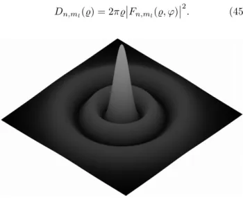
i! . (44) Exemplifying a particular case in Figure 1, we show the probability density of the eigenstate with null angular momentum|F4,0(̺, ϕ)|2. Additionally, in Table 1 we show
the electron radial eigenfunction up to the first six values ofn. In relation to these eigenfunctions, we obtain more
information about every electron eigenstate when we calculate its radial probability density as,
Dn,ml(̺) = 2π̺
Fn,ml(̺, ϕ)
2. (45)
Figure 1:Electron spatial probability density for the eigenstate F4,0. The two concentric darkest rings are associated with
for-bidden radial positions of the electron. The radial distance units are expressed asβ−1, or reciprocal to magnetic field strength as
p
2~/eB.
Table 1:Radial eigenfunction common to the two-dimensional harmonic oscillator and the observableLˆz, for the first six values
ofn. Negative angular momentum projectionmlentails negative azimuthal phase.
n ml Fn,ml(ρ, ϕ) 0 0 F0,0=
β
√πe−β
2
ρ2
/2
1 1 F1,1=
β
√
π(βρ)e
−β
2
ρ2
/2
eiϕ
2 2 F2,2=
β
√ 2π(βρ)
2
e−β
2
ρ2
/2
ei2ϕ
0 F2,0=
β
√π
(βρ)2 −1
e−β
2
ρ2
/2
3 3 F3,3=
β
√ 6π(βρ)
3
e−β
2
ρ2
/2
ei3ϕ
1 F3,1=
β
√ 2π
(βρ)3 −2(βρ)
e−β
2
ρ2
/2
eiϕ
4 4 F4,4=
β
2√6π(βρ)
4
e−β
2
ρ2
/2
ei4ϕ
2 F4,2=
β
√ 6π
(βρ)4 −3(βρ)
2
e−β
2
ρ2
/2
ei2ϕ
0 F4,0=
β
√ 4π
(βρ)4 −4(βρ)
2 + 2e−β
2
ρ2
/2
5 5 F5,5=
β
2√30π(βρ)
5
e−β
2
ρ2
/2
ei5ϕ
3 F5,3=
β
2√6π
(βρ)5−4(βρ) 3
e−β
2
ρ2
/2
ei3ϕ
1 F5,1=
β
√ 12π
(βρ)5 −6(βρ)
3
+ 6(βρ)e−β
2
ρ2
/2
eiϕ
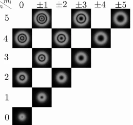
Thus, in Figure 2 we show the radial probability densities of every eigenstates belonging to the first six values ofn.
We want to briefly mention a close relationship between the radial eigenfunction of the electron and Quantum Op-tics. These eigenfunctions are the same as those we can obtain as a natural solutions of the wave equation under the paraxial approximation [19,20], for a Gaussian beam of light in cylindrical coordinates. Commonly, in quan-tum optics these functions are called Laguerre-Gaussian modes, which are expressed through the generalized La-guerre polynomials L|pl|, where p≥0is the radial index
which is related to the number of rings in the probability density of every eigenfunction; we can notice this number in Figure 2 along every diagonal from lower left to upper right. The integer l which is the azimuthal index, has
the same physical meaning as the axial electron angular momentum.
Figure 2:Electron radial probability density of eigenstates be-longing of the first six values ofnand its individual set ofml, in which the radial distance units are expressed asβ−1. All of
these densities showing a null probability of finding the electron in the center position and some well defined rings, where the amount of these rings is(n−|ml|)/2, which is equivalent to the
number of roots of the generalized Laguerre polynomials.
We can obtain the Schrödinger equation in cylindrical coordinates by using the full definition of the electron wave function,
h ˆ
Hρϕ′ + ˆ
p2 z 2m0 +
~ω Lz+2SziFn,m le
ipzz/~Γ
=E Fn,mle ipzz/~Γ.
(46)
We can further obtain the total energy of the electron in relation to its eigenstates,
E= p 2 z 2m0
+~ω n+ml+ 2ms+ 1, ω= eB 2m0
. (47)
In general, the electron energy levels areE≥0, where the zero of energy is associated to eigenstates with a null linear momentumpz, the lowest possible projection
of angular momentumml=−n, and a spin orientation
opposite to the magnetic fieldms=−1/2. Additionally,
under some of the last conditions, we can obtain the energy levels associated to the spin interaction with the external magnetic field as we shown in section 2. However, in this case we see the contribution of the zero-point energy which is related to the harmonic potential; this is the reason for this energy shift.
E= e~B 2m0
(2ms+ 1). (48)
Furthermore, we notice that the addition ofn andml
is always an even number. We can then rewrite the expression for the energy using a new integer number,
E = p 2 z
2m+~ω 2r
, r= 0,1,2,3, . . . n+ml+ 2ms+ 1 = 2r,
(49)
whereris associated to every energy level and is known as
theLandau level. We can see easily that eigenstates with
the same spatial probability density belong to different energy levels. For instance, F1,1 and F1,−1 are associ-ated to different energies, but their spatial probability densities are equal. In general we have,
Fn,ml
2=Fn,−ml
2, En,ml6=En,−ml. (50) In relation to Eq. (49), we can see that every Landau Level is highly degenerate, because the electron eigen-states with different quantum numbers n and ml are
related to the same energy level, as we see in Figure 3. This feature can be observed in the quantization of the cyclotron orbits of charged particles in magnetic field [23]. Such charged particles can only occupy orbits with discrete energy values, but these levels are degener-ate, where the degeneracy is associated to the number of electrons per level. The number of electrons per level is directly proportional to the strength of the applied magnetic field.
Moreover, this physical aspect can be experimentally appreciated within solid materials, where there are elec-tronic oscillations under the action of an external mag-netic field. When we apply a differential of electric poten-tial through the material, this leads to the observation of discrete values of electric current directly related to the Landau levels of the electrons. This phenomenon is commonly called Integer Quantum Hall Effect [24], and its useful applications have been evidenced in quantum metrology in order to acquire more information about microscopic details of semiconductors. Also, evidence of Landau levels has been obtained in the propagation of electron vortex beams along an external longitudinal magnetic field [25].
4. Dirac equation for an electron in
magnetic field
In this section we present the relativistic description, via Dirac equation, for an electron in a region with a uniform magnetic fieldB~. According to this relativistic quantum
description, the electron eigenstate is expressed by the spinorial formalism. In general, a Dirac spinor for the electron is a column vector with four-elements, each one
of which are related to the eigenfunction (42) obtained from the relevant Schrödinger equation. Also, the order of the spinor’s elements are associated with the spin orientation and the energy sign of the electron [26–28], where the energy negative elements are associated to the electron’s antiparticle, commonly called a positron.
After this short description, the electron Dirac equation is,
i~∂
∂tU(~r, t) = cα˜·~pˆ+ ˜βm0c
2U(~r, t), (51) whereU is a general electron spinor. We can write the
linear momentum operator according to the canonical transformation~pˆ→~pˆ+e ~A, whereA~is the magnetic vector
potential. Additionally, we haveα˜ andβ˜which are four
Hermitian matrices with dimension 4×4, satisfying the conditionα˜2= ˜β2= ˆ1,
˜
α=
0 σˆ ˆ
σ 0
, β˜= ˆ
12×2 0 0 −12ˆ ×2
. (52)
Therefore, we obtain the time-independent Dirac Hamil-tonianHˆ=cα˜·p~ˆ+ ˜βm0c2. We can express the electron’s spinor evolution through an unitary transformation,
U(~r, t) =
φ χ
e−i
Et
~, (53)
whereφ andχ are two scalar functions that represent
the first two elements of positive energy and the last two elements of negative energy of the electron’s spinor respectively. When we substitute the spinor (53) in Eq. (51), and using the matrix notation, we obtain,
m0c212ˆ ×2 cσˆ·(−i~∇+e ~A)
cˆσ·(−i~∇+e ~A) −m0c212ˆ ×2
φ χ
=E
φ χ
.
(54) From the first and second row of the matrix we can obtain two linear equations equal to the electron total energy respectively multiplied by the scalar functions defined before,
m0c2φ+cˆσ·(−i~∇+e ~A)χ=Eφ (55a)
cσˆ·(−i~∇+e ~A)φ−m0c2χ=Eχ. (55b)
Isolatingφfrom (55a) and χfrom (55b) yields,
φ= cσˆ·(−i~∇+e ~A)
E−m0c2
χ, χ=cσˆ·(−i~∇+e ~A)
E+m0c2
φ.
(56) Replacingχ byφand vice versa, results in,
E2−m2 0c4
c2 φ=
ˆ
σ·(−i~∇+e ~A)σˆ·(−i~∇+e ~A)φ, =(−i~∇+e ~A)·(−i~∇+e ~A)φ
+iσˆ·(−i~∇+e ~A)×(−i~∇+e ~A)φ.
(57)
The first term on the right is equal to
(−i~∇+e ~A)·(−i~∇+e ~A)φ=−~2∇2φ+e2A2φ −ie~ ∇·A~+A~·∇φ. (58)
Similarly, the second term on the right side of Eq. (57) is equal to
iˆσ·(−i~∇+e ~A)×(−i~∇+e ~A)φ=e~σˆ·(∇×A~) +(A~×∇)φ. (59)
We can then obtain,
∇·A~+A~·∇φ=✟✟ ✟
(∇·A~)φ+A~·∇φ+A~·∇φ,
=2A~·∇φ,
(∇×A~)+(A~×∇)φ= (∇×A~)φ−A~×(∇φ)+A~×(∇φ),
= (∇×A~)φ.
(60)
According to the last results, we rewrite Eq. (57), getting,
E2−m20c4
c2 φ=
−~2∇2+e2A2−2i~e(A~·∇) +e~σˆ·B~φ.
(61)
It’s worth mentioning thate~σˆ·B~ is the term associated
with the interaction potential between the spin of the electron and the external magnetic field. Usually, this term is put in by hand as we, see Eq. (3). This is done in order to ensure a good quantum description when using the Schrödinger equation of an electron with spin1/2in a region with an external magnetic field. On the other hand, this interaction potential appears naturally by using the Dirac equation to describe the same physical system which represents a significant theoretical advantage.
Continuing the analysis, we make a simplification (without loss of physical generality), assuming an ex-ternal uniform magnetic field alongzˆaxis. In this way, we can express the magnetic vector potential by the Lan-dau gauge which allows us to include the axial symmetry as we explained in last section,
~ A= 1
2 −yB, xB,0
. (62)
Replacing the vector potential in Eq. (61) and dividing this equation by2m0yields,
E2−m2 0c4 2m0c2
φ
= "
−~2 2m0
∂2
∂x2+
∂2
∂y2
+e 2B2 8m0
x2+y2
+ eB 2m0
ˆ
Lz+2 ˆSz− ~2
2m0
∂2
∂z2 #
φ.
(63)
harmonic oscillator obtained in the previous section, and a plane wave function of a free particle along the direction of the external field,
φ(~r) =F(x, y)eipzz/~Γ, (64) whereΓ is the spinorial function that we defined previ-ously in Eq. (12). The first two spinor elements, which are related to the positive energy particle, have two spin orientations: up and down. We further have the last two spinor elements which are related to negative energy par-ticle (i.e., an antiparpar-ticle); these are related to the spin orientation similarly. Therefore, we can denote the two positive spinor elements as,
U+(+)1 2
(x, y) =
F(x, y) 0
, U−(+)1 2
(x, y) =
0
F(x, y)
.
(65) When the spin operator acts on the spinor positive energy elements, we obtain the relation,
ˆ
SzUm(+)s(x, y) =~msU (+)
ms (x, y), ms=
+1/2
−1/2 . (66) Furthermore, the commutation relations between the ax-ial angular momentum and the harmonic Hamiltonian are equal to zero, we can say thatLˆzis a conserved physi-cal quantity, and its eigenfunctions are the eigenfunctions of the two-dimensional harmonic oscillator. Thus, we get the following relation,
ˆ
LzUm(+)s(x, y) =~mlU (+)
ms(x, y), (67) whereml is the quantum number of the axial angular
momentum. When we replace Eq. (64) in Eq. (63) we obtain,
E2−m2 0c4 2m0c2
F= "
−~2 2m0
∂2
∂x2+
∂2
∂x2
+1 2m0ω
2 x2+y2+ p2z 2m0
+~ω ml+2ms #
F.
(68)
Rearranging the last equation yields,
" −~2 2m0
∂2
∂x2+
∂2
∂x2
+1 2m0ω
2 x2+y2 #
F
=
E2−m2 0c4 2m0c2 −
p2 z 2m0−
~ω ml+2ms
F,
(69)
from which we notice that the left hand terms in brackets correspond to the Hamiltonian of the two-dimensional harmonic oscillator in Cartesian coordinates with a char-acteristic frequencyω=eB/2m0. Subsequently, we can say that the right hand terms is equal to the energy of the oscillator. We accordingly have,
E2−m2 0c4 2m0c2 −
p2 z 2m0−
~ω ml+2ms
=~ω nx+ny+1. (70)
Due to the total energy being present to the second power, when we isolateE, we obtain two signs for the
total energy of the particle, being the positive sign related to the electron and the negative sign to the positron,
E=± q
m2
0c4+p2zc2+eB~c2 n+ml+2ms+1
. (71)
If we have the particular case of an electron with null lin-ear momentum, an angular momentum projection equal toml=−nand a weak magnetic field in relation to the
rest mass of the electron, then we can approximate the energy expression as,
E≈m0c2
1 + eB~ 2m2
0c2
(2ms+1)
,
=m0c2+
eB~ 2m0
(2ms+1).
(72)
From this, we can obtain the energy levels of the spin interaction with an external magnetic field (as we have shown in the last two sections), the energy shift related to the zero-point energy of the harmonic potential, and the rest mass of the electron, which is relevant by a relativistic description as we done using Dirac equation.
According to the axial symmetry exhibited by the two dimensional harmonic Hamiltonian Eq. (13), we can make a coordinate system transformation in order to rewrite the Hamiltonian in cylindrical coordinates, as we have done in the previous section. We thus obtained the same radial eigenfunctions of the electron, Eq. (42) as those in the case where the electron state is expressed by the Dirac spinor.
Specifically, if we describe the electron using the Dirac equation, we have to consider the first two elements of the Dirac spinor as the radial eigenfunctions obtained in last section. Thus, we implement the relation (56), according to the orientation of the electron’s spin. In the same way, we can obtain the other two elements of the spinor which are related to negative energy states. Then, we express the complete Dirac spinor associated with a particular quantum state of the electron.
To exemplify this process, we calculate a particular case to obtain the Dirac spinor for an electron in a specific state. We choose the ground state of the electronn= 0,
ml= 0 and its spin orientation ms= +1/2. Then, the
electron relativistic energy is,
E0,0= q
m2
0c4+p2zc2+2eB~c2. (73)
Previously, we have obtained the radial wave function of the ground state via Schrödinger equation,
F0,0(̺, ϕ) =
β
√
πe
−β2
̺2
/2, β = r
eB
2~. (74)
We can write the first two elements of the spinor,
U0(+),0 (~r) =
F0,0(̺, ϕ) 0
when we transform the relations (56) in cylindrical coor-dinates.
Firstly, we have to express every unit vector in Carte-sian coordinate as,
ˆ
x
ˆ
y
ˆ
z
=
cosϕ −sinϕ 0 sinϕ cosϕ 0
0 0 1
ˆ
̺
ˆ
ϕ
ˆ
z
. (76)
In this way, the magnetic vector potential is,
~ A=B̺
2 ϕ.ˆ (77)
Similarly, the nabla operator in cylindrical coordinates is,
∇= ˆ̺ ∂ ∂̺+
ˆ
ϕ ̺
∂ ∂ϕ+ ˆz
∂
∂z. (78)
Also, the Pauli matrices vector is written as,
~σ= ˆσxˆx+ ˆσyyˆ+ ˆσzz,ˆ
=
0 e−iϕ
eiϕ 0
ˆ
̺+
0 −ie−iϕ
ieiϕ 0
ˆ
ϕ+
1 0
0 −1
ˆ
z.
(79)
Once we have calculated all the relevant transformations, we are able to use Eq. (56) to calculate the two negative energy elements of the spinor as follows,
cˆσ· −i~∇+eB̺ 2 ϕˆ
E+m0c2 = 1
E+m0c2
−i~c ∂
∂z −2i~cβˆaR
2i~cβˆa† R i~c
∂ ∂z
,
(80) where ˆa†R and ˆaR are the ladder operators defined in
Eq. (37). Therefore, the two electron spinor elements corresponding to the negative energy of the ground state can be expressed as,
U0(,−0)= 1
E+m0c2
cpzF0,0(̺, ϕ) 2i~cβF1,1(̺, ϕ)
eipzz/~. (81)
Therefore, we obtain the complete Dirac spinor associated to the ground state of the electron,
U0,0(~r) =N0,0
F0,0(̺, ϕ) 0
cpzF0,0(̺, ϕ) (E0,0+m0c2) 2i~cβF1,1(̺, ϕ)
(E0,0+m0c2)
eipzz/~, (82)
where its normalization constant is,
N0,0=
1+ c
2p2 z (E0,0+m0c2)2
+ 4~ 2c2β2 (E0,0+m0c2)2
−1 2
. (83)
We would like to emphasize the relevance of the two negative elements of the Dirac spinor for an electron in two specific cases:i) When the electron has a great linear
momentum and it is the dominant physical quantity, we have that the electron speed is very close to the speed of light and the third spinor element becomes relevant for this description.ii) When we have a strong confinement of the electron and it is trapped in a region less than or equal to its Compton wavelength [29,30]. Thereby, the fourth spinor element becomes relevant to the physical description. Thus, we can obtain this last case when the electron is in a region with a very strong magnetic field, yielding a high characteristic frequencyωof the harmonic
potential, as consequence a very small natural length of the harmonic oscillatorp
~/m0ω. As such, we show in
Figure 4 a different radial probability density of the electron ground state via Dirac equation, in comparison to that obtained before via Schrödinger equation.
The fourth element of the spinor shows an excited eigenstaten, ml= 1,1; whose contribution is comparable
to the first element. Subsequently, this element of the spinor becomes relevant for the description of the electron quantum state; and this is why we observe a more open electron radial probability density via the Dirac equation.
We advise to the reader to see a short animation [31] about the radial probability density according to both the-ories in relation to the external magnetic field strength. In summary, we can conclude that the quantum me-chanical description via the Dirac equation requires more complicated mathematical steps, but that it also brings new concepts, such as the negative energy of the elec-tron and a different treatment through the application of Dirac spinors; this yields a more general way to de-scribe the quantum state of an electron when relativistic effects are taken into account which is richer than the Schrödinger description.
Acknowledgements
The first author wish to thank to his doctoral advisor Eduardo, for all fruitful discussions and his great listening and grateful understanding. Finally, the Brazilian agency CAPES for its financial support.
References
[1] E. G. P. Rowe, Am. J. Phys.59, 1111 (1991).
[2] C. Cohen-Tannoudji, B. Diu, F. Laloë, Quantum me-chanics(Wiley, New Jersey, 1991) v. 1, Section VI. [3] T. Haugset, J. A. Ruud and F. Ravndal, Physica Scripta
47, 715 (1993).
[4] D. Yoshioka,The Quantum Hall Effect(Springer, Berlin, 2002) Chapter 2.
[5] B. Thaller, Advanced Visual Quantum Mechanics (Springer, Berlin, 2004).
[6] C. R. Greenshields, R. L. Stamps, S. Franke-Arnold and S. M. Barnett, Phys. Rev. Lett.113, 240404 (2014). [7] M. Babiker, J. Yuan, and V. E. Lembessis, Phys. Rev.
A91, 013806 (2015).
[8] D. Chowdhury, B. Basu, and P. Bandyopadhyay, Rev. A
91, 033812 (2015).
[9] K. Y Bliokh, Y. P. Bliokh, S. Savel’ev and F. Nori, Phys. Rev. Lett.99, 190404 (2007).
[10] L. Landau, Z. Physik64, 629 (1930).
[11] A. Feldman and A. Kahn, Phys. Rev. B1, 4584 (1970). [12] T. Chakraborty, P. Pietiäinen,The Quantum Hall Effect:
Integral and Fractional, (Springer, Berlin, 1995). [13] R. B. Laughlin, Phys. Rev. B23, 5632 (1981).
[14] P. Schattschneider, T. Schachinger, M Stöger-Pollach, S. Löffler, A. Steiger-Thirsfeld, K. Y. Bliokh, F. Nori,5, 4586 (2014).
[15] Ole Steuernagel, Am. J. Phys.73, 625 (2005).
[16] L. Allen, M. W. Beijersbergen, R. J. C. Spreeuw and J. P. Woerdman, Phys. Rev. A45, 8185 (1992).
[17] S. Zhang and Z. Yang, Phys. Rev. Lett. 94, 066602 (2005).
[18] W. E. Baylis, J. Bonenfant, J. Derbyshire and J. Huschilt, Am. J. Phys.61, 534 (1993).
[19] G. Goubau and F. Schwering,9, 248 (1961).
[20] D. L. Andrews and M. Babiker,The Angular Momentum of Light(Cambridge University Press, Cambridge, 2001), 1st edition.
[21] S. Feng and H. G. Winful, Opt. Lett.26, 485 (2001). [22] P. B. Monteiro, P. A. Maia Neto and H. M. Nussenzveig,
Phys. Rev. A79, 033830 (2009).
[23] S.A. Mikhailov, Physica B299, 6-31 (2001).
[24] B. Jeanneret, B. D. Hall, H.J. Bühlmann, R. Houdré, M. Ilegems, B. Jeckelmann and U. Feller, Phys. Rev. B51, 9752 (1995).
[25] K. Y. Bliokh, P. Schattschneider, J. Verbeeck and F. Nori, Phys. Rev. X2, 041011 (2012).
[26] P. Strange,Relativistic Quantum Mechanics with appli-cations in condensed matter and atomic physics (Cam-bridge University Press, Cam(Cam-bridge, 1998), 1st edition. [27] W. Greiner,Relativistic Quantum Mechanics wave
equa-tions, (Springer, Berlin, 2000), 3rd edition.
[28] B. H. Bransden and C. J. Joachain,Quantum Mechanics, (Prentice Hall, New Jersey, 2000), 2nd edition.
[29] C. C. Leary and Karl H. Smith, Phys. Rev. A89, 023831 (2014).
[30] D. V. Villamizar and E. I. Duzzioni, Phys. Rev. A92, 042106 (2015).