www.hydrol-earth-syst-sci.net/16/3061/2012/ doi:10.5194/hess-16-3061-2012
© Author(s) 2012. CC Attribution 3.0 License.
Earth System
Sciences
Combining ground-based and airborne EM through
Artificial Neural Networks for modelling glacial till
under saline groundwater conditions
J. L. Gunnink1, J. H. A. Bosch1, B. Siemon2, B. Roth3,*, and E. Auken3
1Geological Survey of The Netherlands TNO, The Netherlands
2Federal Institute for Geosciences and Natural Resources (BGR), Germany 3Department of Geosciences, Aarhus University, Denmark
*now at: Aarhus Geophysics Aps, Denmark
Correspondence to:J. L. Gunnink ([email protected])
Received: 29 February 2012 – Published in Hydrol. Earth Syst. Sci. Discuss.: 13 March 2012 Revised: 26 July 2012 – Accepted: 6 August 2012 – Published: 29 August 2012
Abstract.Airborne electromagnetic (AEM) methods supply data over large areas in a cost-effective way. We used Artifi-cial Neural Networks (ANN) to classify the geophysical sig-nal into a meaningful geological parameter. By using exam-ples of known relations between ground-based geophysical data (in this case electrical conductivity, EC, from electrical cone penetration tests) and geological parameters (presence of glacial till), we extracted learning rules that could be ap-plied to map the presence of a glacial till using the EC pro-files from the airborne EM data. The saline groundwater in the area was obscuring the EC signal from the till but by us-ing ANN we were able to extract subtle and often non-linear, relations in EC that were representative of the presence of the till. The ANN results were interpreted as the probability of having till and showed a good agreement with drilling data. The glacial till is acting as a layer that inhibits groundwater flow, due to its high clay-content, and is therefore an impor-tant layer in hydrogeological modelling and for predicting the effects of climate change on groundwater quantity and quality.
1 Introduction
Management of surface water and groundwater in deltaic ar-eas is of paramount importance to sustain the current land use and to protect the inhabitants from flooding, either by the sea, rivers or groundwater (CLIWAT, 2011). In deltaic areas,
with surface levels around or below mean sea level (m.s.l.), the groundwater is often saline due to seawater intrusion and marine transgressions in the past. Climate change predictions of increasing seawater levels and precipitation (especially in wintertime) will likely affect the groundwater flow and groundwater quality, especially the salinisation of groundwa-ter (de Louw et al., 2011). To be able to forecast the effects of climate change, spatially distributed groundwater flow mod-els (both quantity and quality) are needed. These modmod-els re-quire input parameters (hydraulic conductivity, porosity etc.) that vary in 3-D space, and are based on the geological his-tory of the modelled area. The usual workflow is to create a geological model that is subsequently converted to a ground-water flow model by selecting aquifers and aquitards from the geological model and assigning the appropriate hydro-logical parameters.
Fig. 1.Location of the study area, ECPTs and airborne geophysical data.
a large area in a cost-effective way. One of the most popular techniques used in groundwater studies is the electro mag-netic (EM) method that results in a quasi-3-D model of the resistivity of the subsurface (Kirsch, 2009). EM resistivity (and its reciprocal, conductivity) might give an indication of the geological build-up of the subsurface, when the resistivity can be linked to lithological variation.
In this paper we describe techniques to combine 1-D (point) data and quasi-3-D proxy data to produce a geolog-ical model of the subsurface that can be used for hydroge-ological modelling. Robinson et al. (2008) recognized the need for improved geophysical measuring systems and sub-sequent conversion of the geophysical signal to geological and hydrogeological meaningful parameters that can be used in distributed watershed modelling. Geostatistical methods of interpolating in between boreholes require a representative dataset that is often not available, due to the limited amount of drillings and the large distances between the drillings. For the proxy data to be useful in geological modelling, it is necessary to convert the geophysical signal into a geo-logical parameter (Gunnink and Siemon, 2009; Bosch et al., 2009). This can be seen as a classification problem, for which artificial intelligence is well suited.
2 Study area
The study area is located in the northern part of Fryslˆan, the Netherlands (Fig. 1). This area is one of the pilot ar-eas of the CLIWAT project (www.cliwat.eu), and several geophysical techniques were employed, both airborne, HEM (frequency domain airborne electromagnetics) and SkyTEM (time-domain airborne EM), and land-based, electrical cone penetration test, (ECPT). The main land use in the area is grassland and agriculture. The average surface level is around mean sea level, and is measured relative to the Dutch Or-donance Level (NAP). In the area fluvial sediments, mainly consisting of sand and occasionally clay were deposited in the Early and Mid-Pleistocene (Peize-Waalre (PZWA),
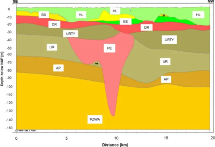
Ap-Fig. 2. SE-NW geological cross section, showing the main geo-logical units; PZWA: Peize/Waalre formation; AP: Appelscha for-mation; PE: Peelo formation (from Elsterian glaciation); UR: Urk formation; URTY: Urk-Tynje formation; DR: Drente formation (Saalian glaciation); EE: Eem formation; BX: Boxtel formation (Weichselian glaciation); HL: Holocene formations.
pelscha (AP) and Urk (UR) Formations). In the Elsterian, some tunnel-valleys were formed and were filled with sand, sometimes capped by clay (Peelo Formation (PE)). No tills from this time period are found in the area. After the El-sterian, fluvial deposits were again dominant (Urk-Tynje (URTY) formation) until the land ice reached the area in the Saalian ice age and a till layer at approx. 10–30 m depth was deposited (Drente Formation (DR)). The till covers the en-tire area and dips slightly to the north-west. Its thickness is erratic and can vary considerably over short distances. The till is considered to be an important layer in the groundwa-ter flow, due to its low hydraulic conductivity. Afgroundwa-ter the land ice retreated, a marine transgression caused the sedimenta-tion of sand and clay (Eem Formasedimenta-tion (EE)). Another ice age (the Weichselian) did not produce land ice in the area but widespread aeolian coversands, the Boxtel Formation (BX)). The latest (Holocene (HL)) transgression produced a sequence of alternating sand and clay deposits (with locally some peat) ranging from more than 10 m in the north-west to less than 2 m in the south-east. For extensive description of the geological formations see Mulder et al. (2003).
In large parts of the study area the groundwater is saline, with the boundary between brackish and saline less than 5 m below surface level. Only in the southeastern part of the area the groundwater is fresh.
3 Materials and methods
3.1 Drillings
The National Database of the Geological Survey of the Netherlands/TNO (www.dinoloket.nl) contains (amongst other data types) drillings that are stored and described in a consistent way. In the study area more than 3900 drillings are available, although more than 90 % of them only sample the upper 5 m. For only a small amount of the drillings men-tioned above, the geological formations were determined, in which the glacial till is especially of interest for this study.
3.2 ECPT
For this project, 71 ECPTs were carried out. Cone penetra-tion tests are originally devised to establish the strength of the sediments in geotechnical engineering. A sleeve of about 0.2 m with a cylindrical shaped conus is pushed into the soil with a constant speed. The resistance of the conus is mea-sured, together with the friction alongside the sleeve. When pushed into the soil, every 0.02 m a measurement is taken. The Electrical CPT also measures the electrical conductivity by means of electrodes that are installed in the conus. For an extensive description of CPT’s see Lunne et al. (1997). Clas-sification of CPTs into lithological units (clay, sand, peat, etc.) can be done with standard tables that are adapted to local geology. The ECPTs in this study were classified into geolog-ical formations based on the cone resistance and sleeve fric-tion and the regional knowledge of the geology. This leads to a dataset with depth of the top and bottom of each for-mation and its electrical conductivity (EC). In Fig. 3 some typical examples are given of the variation of the electrical conductivity with depth, combined with data regarding the occurrence of geological strata. For clarity reasons, the geo-logical formations are grouped into 4 major units: Holocene formations, post-Saalian formations (deposited on top of the glacial till), the glacial till and the pre-Saalian formations. The EC is dominated by the saline groundwater, resulting in high conductivities compared to, for example, the sur-face layers where the groundwater is fresh. In Fig. 3 the EC is constantly increasing with depth (up to the glacial till sediments), regardless of the lithological composition. The boundary between the Holocene sediments (mixture of sand and clay) and the underlying post-Saalian sediments (sand) is not noticeable, except for ECPT S05G00606 and ECPT S05G00609. Furthermore, the alternations of clay and sand in the Holocene sediments (not shown in the graph) do not show up in the EC profile. This is due to the large influence of the saline groundwater on the EC, which obscures the effects of lithological composition on the EC. On the other hand, it can be noted that there is a drop in electrical conductivity in the interval in which the glacial till occurs. Inspection of all ECPTs revealed that in the majority of the ECPTs in which the glacial till was found it showed a similar behaviour:
de-creasing EC in the depth-interval of the till, although the ac-tual decrease in EC and its magnitude is not uniform. The reason for this lower EC is not clear: the glacial till is clayey, which theoretically causes a higher conductivity compared to the sandy sediments below and above the till. A possible rea-son for the lower electrical conductivity might be the water quality in the till, which could be more fresh than the sur-rounding sandy sediments. The last transgression caused the salinisation of the groundwater, but due to the clayey nature of the till and consequently low hydraulic conductivity, not all (initial) fresh water is possibly replaced by saline water. Since there are no groundwater samples from the till, this unfortunately cannot be validated.
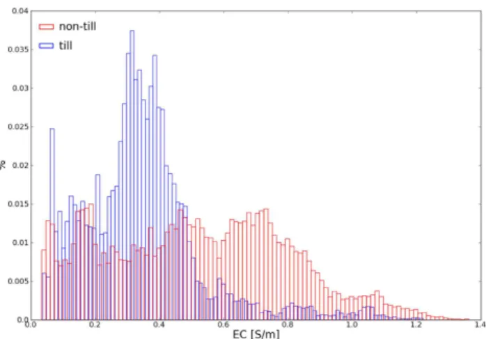
For all ECPTs combined, the EC of the till interval was compared to the EC of the layers above and below the till. In Fig. 4 the combined histogram of EC for till and non-till is shown. There is some overlap in the two distributions, but it is also clear that there is a distinction between the statistical distribution of the EC of the till and the EC of the non-till. This underpins the observed EC distinction between till and non-till, as seen in the individual ECPTs.
3.3 Airborne EM
The study area was covered by two airborne EM surveys us-ing helicopter-borne frequency domain (HEM) and time do-main (SkyTEM) systems often used in groundwater studies (Siemon et al., 2009b; Steuer et al., 2009). In a small part, the two surveys overlapped (see Fig. 1). The data processing of the airborne EM is described extensively in the next sections, because the processed EM data serves as the main input for the subsequent analyses to model the glacial till.
3.3.1 HEM
Frequency domain EM methods are able to measure both the induced secondary magnetic field and the inducing primary magnetic field generated by a sinusoidal varying source cur-rent. The latter is generally cancelled out so the method be-comes sensitive to the conductivity distribution in the subsur-face. Furthermore, the complex secondary field is normalised by the primary field at the receiver. HEM methods use circu-lar transmitter, receiver, bucking and calibration coils which are rigidly mounted in horizontal coplanar (HCP) or verti-cal coaxial (VCX) orientation in the bird. The HEM sys-tem used in the Fryslˆan survey is a Resolve syssys-tem consist-ing of five HCP and one VCX coil systems. Transmitter-receiver separations are about 7.92 m and 9.06 m, respec-tively. The frequencies range from 386 Hz up to 133 kHz en-abling investigations down to about 150 m in resistive (about >100 Ohm m−1) and 50 m in conductive grounds (about<
10 Ohm m−1). In the presence of saline groundwater and
Fig. 3.Geological variation and EC, as derived from ECPT.
Fig. 4.Distribution of EC for intervals with and without glacial till.
has been successfully applied in a number of groundwater surveys in recent years (Siemon et al., 2007, 2012; Steuer et al., 2008; de Louw et al., 2011; Sulzbacher et al., 2012).
3.3.2 HEM survey
In the study area, a helicopter-borne survey was conducted by the BGR airborne group in August 2009 (see Fig. 1 for lo-cation). The airborne survey comprises an area of nominally 5–10 km by 12–24 km, which was flown with 6 survey flights totalling about 616 line-km. The nominal flight-line spacing was 250 m for the 41 ENE–WSW profile lines and 2000 m for the 8 NNW–SSE tie lines. A radar station for air-traffic control strongly disturbed the airborne measurements, hence an area of about 7 km by 10 km in the centre of the planned survey area could not be covered (Siemon et al., 2010).
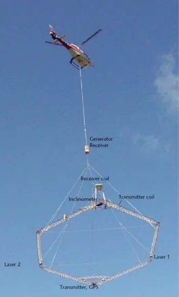
The BGR helicopter-borne geophysical system (Fig. 5) si-multaneously records six-frequency electromagnetic, mag-netic and radiometric data. Besides the electromagmag-netic and magnetic sensors, the GPS antenna and a laser altimeter are installed inside the towed tube called bird. The navigation instruments and the gamma-ray spectrometer are mounted in the helicopter. A ground base station records the time-variant data required to correct the airborne data. The survey alti-tudes of the towed sensors are normally 30–40 m. Data are recorded 10 times per second. At an aircraft speed of about 140–150 km h−1leads to a mean sampling interval of about
4 m. Due to the relative high conductivity in the subsurface of the survey area, the maximum HEM depth of investiga-tion ranges from about 30 m in the south-west area to about 100 m in the north-east area.
3.3.3 HEM data processing
Fig. 5.The BGR helicopter-borne geophysical system.
responses of individual soundings were inverted, based on the Marquardt-Levenberg approach, to layered models with five layers (Sengpiel and Siemon, 2000; Siemon et al., 2010) using individual starting models derived from apparent resis-tivity vs. centroid depth sounding curves (Siemon, 2001). A comparison with ECPT data showed that the use of smooth fifteen-layer models provided better results (Mitreiter and Siemon, 2011). Therefore, the smooth-layer approach was used to include a-priori ECPT data to constrain the HEM in-version. For this, the Laterally Constrained Inversion (LCI, Auken et al., 2005) approach applied to HEM data (Siemon et al., 2009a) has been modified to automatically include ECPT conductivities as prior data.
All the already existing starting models close to an ECPT site (i.e. within the search radius) are replaced by the cor-responding ECPT model, but only down to the maximum depth of an ECPT plus 10 %. Besides these prior constraints, lateral and vertical constraints are used by the LCI to find a reasonable balance between the importance of HEM and ECPT data. The most promising results could be achieved for a smooth inversion with fifteen layers using a search ra-dius of 250–500 m and depth dependent vertical and lateral constraints on the resistivities, i.e. the resistivities were
con-Fig. 6.SkyTEM helicopter system.
strained to 100 % (vertical) and 10 % (horizontal) change at the shallowest depth and to 10 % (vertical) and 1 % (hori-zontal) change at the greatest depth. In this case we used 5 times decimated dataset resulting in a sounding distance of about 20 m.
3.3.4 SkyTEM
Transient Electromagnetic Methods (TEM) measure the in-duced or secondary electromagnetic field due to the diffu-sion of the eddy currents in the ground after the source cur-rent is turned-off. Examples of mapping of groundwater re-sources are reported in Auken et al. (2010), Kafri and Gold-man (2005), Kok et al. (2010).
with two moments, one called Super Low Moment (SLM, ∼3100 Am2)which gives information of the near surface, and one called High Moment (HM,∼122 000 Am2)which gives deep information. These two moments are jointly in-verted for each single sounding estimating electrical resistiv-ity from the near-surface to a depth of 250–300 m, depending on the setup used and the overall formation resistivity in the survey area.
Data are corrected for pitch and roll from frame move-ments in the airspace (by inclinometers mounted on the frame) and the height above the ground is included in the inversion with an a-priori measured one by lasers mounted on the frame (Auken et al., 2009).
3.3.5 SkyTEM survey
The SkyTEM survey was carried out in the period 14– 18 September 2009. The survey consists of approximately 1000 line km of data with a line spacing of 200 m and covers an area of 225 km2(see Fig. 1). The SkyTEM survey utilised a small loop with an area of 282 m2and 4 turns aiming for increased resolution of near surface geology rather than max-imizing depth of investigation. The first time gate on SLM (calculated from begin of the turn off ramp) was in 12 µs, while the last gate on HM was in 21 ms. Coil correction was applied to the early time gates resulting in a first SLM gate at 8 µs. An average sounding was produced for each 25–30 m, ensuring that the raw data is not averaged over distances greater than the distance between the individual soundings. At later gates the lateral average was increased in order to enhance the depth of investigation. With this setup and the relative low resistive layers in the survey area, the resolution ranges from a few metres below the surface to about 100 m in the north-west area and 250 m in the south-east area. 3.3.6 SkyTEM data processing
The data were processed and inverted with the Aarhus Work-bench software package (Auken et al., 2009). A major part of the processing time was spend on removal of disturbed data due to coupling to pipes, wires, etc. on the ground (Sørensen et al., 2001). The survey areas have a dense infrastructure and about 25 % of the data had to be removed, still leaving more than 29 300 soundings for the geological modelling. Data were inverted using the Spatially Constraint Inversion (SCI) algorithm which gives a quasi-3-D interpretation of the geo-logical layers (Viezzoli et al., 2008, 2009). Each model was a 25 layer smooth model with logarithmic increasing layer thickness in the interval from 2–32 m, with a maximum depth of 240 m. At the end of the inversion, the depth of inves-tigation (DOI) (Christian and Auken, 2010) was calculated allowing to estimate to what depth the EM field contains in-formation on the resistivity. For all details of the setup of the SkyTEM system, the exact processing and inversion settings we refer to Roth et al. (2011).
To further increase the resolution we added a-priori infor-mation to all TEM models in a radius of 200 m from the lo-cation of the ECPT. The a-priori resistivity of each layer in the TEM model was calculated as the integrated conductivity of the corresponding interval in the ECPT, while the standard deviation (STD) on the a-priori value was set to a factor of 1.1 from 0–50 m from the ECPT and then decreasing with the square of the distance from 50–200 m ending at a factor of 1.0, i.e. the allowed deviation of the model conductivities from the ECPT values was 10 % and 10–100 %, respectively.
3.4 Comparing airborne EM with ECPT
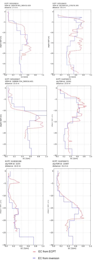
Fig. 7.Some selected examples of comparison between EC from ECPT and EC from airborne HEM and SkyTEM models (within 50 m), without a-priori constraints.
considerable lateral variation. Figure 10 shows the effect of using a-priori EC data from the ECPT, while Fig. 11 shows the EC distribution with depth for the cross sections indicated in Fig. 1.
4 Artificial Neural Networks
4.1 Introduction into ANN
Artificial Neural Networks (ANN) are a form of artificial intelligence that attempts to mimic the function of the hu-man brain and nervous system (Aminzadeh and de Groot, 2006). ANN learn from data examples presented to the al-gorithm and it is capable of capturing subtle relationships in the data, even if the underlying (physical) relationships are unknown or difficult to explain. The advantage of ANN over traditional empirical and statistical methods is that there is no need to introduce prior knowledge about the nature of the re-lationship among the data. ANN are therefore well suited to modelling the complex, often non-linear behaviour of earth science data, which by their nature often exhibit large vari-ability. Examples are the use of ANN in classifying lithology (Bhattacharya and Solamatine, 2006), improving parameter extraction from geophysical data for hydrological modelling (Hinnel et al., 2010) and deriving parameters from Remote Sensing data (Krasnapolsky and Schiller, 2003).
The structure and operation of ANN have been described in detail by numerous authors (Shahin et al., 2008; Sandham and Legget, 2010). We will only discuss the basics of ANN here; the interested reader is referred to standard textbooks like Hsieh (2009).
ANN consists of a number of artificial neurons, called units, nodes or perceptrons. In earth science application, Multi Layer Perceptrons (MLP) is the most commonly used, in which the processing elements are usually arranged in lay-ers: an input layer, an output layer and one or more interme-diate layers, called hidden layers (Fig. 12a), and its operation is given by Eqs. (1) and (2).
Ij=θj+ Xn
i=1wj ixi (1)
yj =f (Ij) (2)
whereIj is the activation level of nodej,wj iis the connec-tion weight between nodes i and j,xi is the input from node i=1,. . . n,θj is the threshold for nodej,yj is the output for nodej andf (.)is the transfer function.
Fig. 8. (a)Comparison between Ln(EC) of airborne models (HEM and SkyTEM) and average Ln(EC) from corresponding interval in the ECPT. Maximum distance between airborne EM model and ECPT is 50 m.(b)Comparison between Ln(EC) of airborne models (HEM and SkyTEM), using a-priori ECPT data, and average Ln(EC) from corresponding interval in the ECPT. Maximum distance between EM model and ECPT is 50 m.
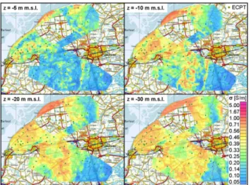
Fig. 9.Depth slices of EC from HEM and SkyTEM models.
The propagation of information in MLP starts at the input layer, where the input data are presented. The next layer re-ceives the weighted inputs from each node in the input layer and the weights are summed and passed through a transfer function to produce the nodal output, which is then weighted and passed to neurons in the next layer. The network ad-justs its weights by using a learning rule until it finds a set of weights that will produce the input-output mapping with the smallest possible error. This process is called the learning or training stage.
In general, the data is split in at least two parts, a learning dataset and a dataset on which the learning rule is tested.
4.2 Application of ANN
Fig. 10.Comparison between HEM inversions without and with a-priori constraints from ECPTs. Location of cross section is C-C’, see Fig. 1.
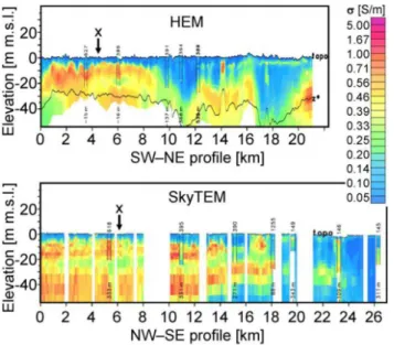
Fig. 11.Cross sections showing the EC for HEM (upper figure, cross section B-B’) and SkyTEM (lower figure, cross section A-A’) inversions with a-priori constraints of ECPTs. For location of cross sections, see Fig. 1. The black line in the upper figure denotes the centroid depth values (Z∗), indicating the depth of investigation.
EC in the airborne models and the ECPTs are comparable, we can use the training on the Ln(EC) of the ECPTs for the Ln(EC) of the airborne EM models.
4.2.1 Data pre-processing
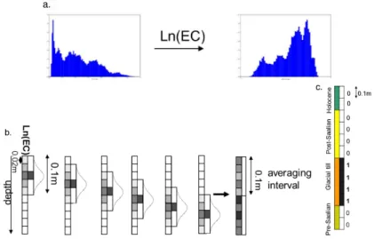
The selection and pre-processing of the input data is a crucial step in the successful application of ANN. The procedure is described in detail here using Fig. 13.
Fig. 12. (a)Typical layout of Artificial Neural Network (ANN) ar-chitecture.(b)Activation of transfer function in ANN.
a. In order to normalise the distribution of the EC and thereby enhancing the discrimination capabilities be-tween different EC-intervals (till vs. non-till) in the ANN, Ln(EC) was calculated. All subsequent process-ing and calculations were carried out for the Ln(EC) data.
b. A smoothing algorithm was used to filter out the noise from the data. A moving window of 0.1 m was used, in which the data points at the border of the window re-ceived less weight than the data points in the middle of the window, according to a Gaussian weighting distribu-tion scheme. Aggregadistribu-tion into 0.1 m intervals was done by simply averaging the smoothed Ln(EC) over 0.1 m. c. For every interval of 0.1 m in the ECPT, the occurring
geological formations, as determined from the sleeve and tip friction of the ECPTs, was ascribed to that in-terval. In this way, for each interval of 0.1 m, the ln(EC) and the occurring geological formation is known. Since the focus of the study is on determining the glacial till, all intervals in which the till was determined were la-belled 1, the remaining intervals were lala-belled 0; this is the in following interpreted as the probability of en-countering till.
The result of the data processing is a dataset that has a depth-interval of 0.1 m, in which each depth-interval has a Ln(EC) and the probability of till.
4.2.2 Training and testing the ANN
Fig. 13.Data pre-processing for training the ANN.
consist of the Ln(EC) value and the depth at every 0.1 m in-terval of the ECPT (see Fig. 13c). The depth was used in or-der to account for the general trend in depth of the glacial till, dipping to the north-west. We experimented with the amount of nodes in the hidden layer and selected three nodes. The network layout is given in Fig. 14, together with the search algorithm.
Because of the general dipping of the depth of the till, it was decided that it is not meaningful to use one trained net-work for the entire area. Therefore, the training of the ANN was made location dependent, so that the changing depth of the till could be accounted for.
For every airborne EM model, a maximum of 3 closest ECPTs were selected and used to train the local network. To account for the fact that some EM models are close to an ECPT, it was decided to make the number of ECPTs to be used in the training of the ANN depending on the distance to the EM model. If the distance between the EM model and the ECPT was less than 250 m, the closest ECPT was used. If the distance between the EM model and its surrounding ECPTs is between 250 m and 1000 m, the algorithm searches for the two closest ECPTs between 250 m and 1000 m, while with distances greater than 1000 m the three closest ECPTs were used (see Fig. 14). To select a maximum of three ECPTs to train the network was a trade-off between enough data to train the network and trying to make the trained network as local applicable as possible. The ECPT cover well the study area, which helped considerably to obtain good trained net-works for the study area.
We used the ANN algorithm developed in the Python pro-gramming language by Wojciechowski (2009). This algo-rithm is designed using feed-forward architecture, with iden-tity functions for the input nodes and sigmoid activation functions for all other neurons. The function that is min-imised during training is a sum of squared errors of each output for each training pattern.
The next step in the general procedure of applying ANN is to test the network. Since we are using only a limited amount of ECPT data for every training (maximum the 3 closest) it was decided it was not feasible to set aside a part of this lim-ited amount of data to test the network. Instead, to determine the goodness of fit when the trained network is applied to the models of the airborne EM, we selected drillings in the area that were classified as having till. The top and bottom of the till from the drillings was used to test the results of the ANN network of the closest (<75 m) airborne EM model.
The network that is trained with the data of the ECPTs will be used to obtain an estimate of the presence and depth of the glacial till from the airborne EM models. The airborne EM models were processed and inverted with a pre-defined layer thickness that increases with depth. For every layer of the inversion, the mid-depth was chosen as representative for its depth, as well as the Ln(EC).
The ANN procedure might result in probabilities smaller than 0 or larger than 1. If this occurred, we arbitrarily set the probabilities to 0 and 1, respectively.
Fig. 14. (a)Neural Network architecture for determining till from Ln(EC) and depth. (b) Search strategy for determining relevant ECPTs for training ANN.
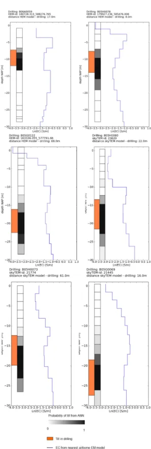
right lower corner in Fig. 16. The bottom of the till is more difficult to estimate: the ECPTs often only reached the bot-tom of the till and did not enter deep enough in the underlying sediments, thereby not capturing the full pattern of the EC with depth. Also there are less drillings that reached the bot-tom of the till compared to drillings that reached the top.
In 8 out of the 21 SkyTEM models (38 %) that were within 75 m of a drilling, the ANN did not detect the top of the till with a probability larger than 0.75. The results of the ANN on these 8 EM models were inspected more closely and it was found that 5 of them were more than 55 m from the near-est drilling or showed a till thickness less than 2 m, which is the approximately layer thickness of the SkyTEM inversion model at that depth. Two out of the 8 EM models did have the top of the till estimated within 1 m of the top of the till in the nearby drilling, only with a probability slightly less than 0.75 (with a minimum probability of 0.65).
For the HEM models that were closest to a drilling (within a maximum of 75 m), 6 out of 15 models did not detect the till at a probability>0.75. Inspection of the results of the ANN applied to these HEM models shows that the probability at which the till was detected was only slightly lower than 0.75, with a minimum of 0.7. Only for 2 out of 15 (13 %) HEM models that were located within 75 m of a drilling, the top of the till was not detected with a probability>0.7.
Fig. 16.Comparing top and bottom of till, as determined from ANN with top and bottom of the till in closest drilling (max. distance 75 m); (a)top of the till from HEM,(b) top till from SkyTEM,
(c)bottom of the till from HEM and(d) bottom of the till from SkyTEM. Correlation coefficient is given in the right-lower corner of each figure.
Regarding the bottom of the till, the correlation for both HEM and SkyTEM models between the bottom of the till in the drilling and from the models is weaker. Also, the bottom of the till suffers from the same problem with the pre-defined threshold of 0.75: more than half of the models did not detect the till at a probability of>0.75, but did so at a probability between 0.6 and 0.75. In a case where the thickness of the till is less than 2 m, the airborne EM could not detect differ-ences in EC and therefore the ANN was not able to produce a probability of having till. Besides this, sometimes the bottom of the till was not detected because it was deeper than in the surrounding ECPTs that were used for training the ANN. 4.3 Applying the ANN to airborne EM
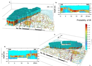
For every model of both HEM and SkyTEM, the ANN pro-cedure, as described above, is applied to obtain the prob-ability of till. For every EM model, the closest 3 ECPTs were selected and the ANN was trained with the data from these ECPTs and subsequently the trained network was ap-plied to the EM model. This resulted in a probability of till for each interval in the EM model. These probabilities were then interpolated over the entire area to a voxel model of 50×50×1 m. For every voxel, the probability of having till is then known. The resulting 3-D model is shown in Fig. 17, together with cross sections that are situated at the same lo-cation as the airborne EM cross sections of Fig. 1.
Fig. 17.3-D voxel models of the probability of till, as derived from ANN of HEM and SkyTEM models.(a)and(b)are derived from SkyTEM models,(c)and(d)from HEM models. Cross section(b)
is A-A’ in Fig. 1; cross section(d)is B-B’ in Fig. 1.
The general trend of the till is in agreement of what is known of the till from the drillings, which is also true for the estimate of the top of the till. The bottom of the till shows some noisy features that are probably due to artefacts. On the other hand, it is known that the bottom surface of the till is erratic and can show large fluctuations over short distances.
The results of the modelling of the glacial till are used in a subsequent study that models the effects of climate change on the groundwater system, with an emphasis on salinisa-tion (Faneca S`anchez et al., 2012). This study shows that the glacial till is an important aquitard, inhibiting groundwater flow and therefore an important spatial feature that should be modelled as accurately as possible.
5 Conclusions
Airborne geophysics, combined with ground-based data proved to be a useful tool for mapping a regional glacial till layer in a highly conductive environment. The till layer is an important hydrological layer because it acts as an aquitard inhibiting groundwater flow. The till layer shows a large spa-tial variability in thickness and is therefore not easily mapped with conventional data (drillings, CPT). Due to the distinct pattern of conductivity of the till in ground-based ECPTs, and the good agreement between airborne and ground-based conductivity profiles, this distinct pattern of conductivity in the ECPT served as a training set for the recognition of the till in the airborne EM results.
modelling to predict the effects of climate change on, for ex-ample salinisation. Because of its widespread occurrence and its erratic top and bottom, it is important to map the till layer as detailed as possible, in order to obtain sound predictions of the effect of climate change on salinisation of groundwater.
The use of ANN to discriminate between different sedi-ments by (airborne) EM is depending on the specific pattern of the Electrical Conductivity for the sedimentary sequences in the study area. Field data of EC, together with sedimen-tary interpretation is therefore essential, together with the understanding of the geology of the area. This combination should lead to a balanced training dataset, in which geologi-cal and geophysigeologi-cal knowledge are combined to achieve the best result possible.
Acknowledgements. This study was part of the Intereg IVb project Cliwat (www.cliwat.eu), co-sponsored by the North Sea Programme of the EU. We thank Wilbert Elderhorst (Province Fryslˆan) and Joca Janssen (Waterboard Fryslˆan) for their fruitful cooperation. Angelika Ullmann and Ivonne Mitreiter are thanked for processing and evaluating the HEM data, Rik Noorland is thanked for his work on the SkyTEM inversions. The members of the CLIWAT project team are acknowledged for their stimulating discussions.
Edited by: H. Wiederhold
References
Aminzadeh, F. and de Groot, P.: Neural Networks and other soft computing techniques with applications in the oil industry, EAGE Publications, The Netherlands, 2006.
Auken, E., Christiansen, A. V., Jacobsen, B. H., and Foged, N.: Piecewise 1-D laterally constrained inversion of resistivity data, Geophys. Prospect., 53, 497–506, 2005.
Auken, E., Christiansen, A. V., Westergaard, J. A., Kirkegaard, C., Foged, N., and Viezzoli, A.: An integrated processing scheme for high-resolution airborne electromagnetic surveys, the SkyTEM system, Explor. Geophys., 40, 184–192, 2009.
Auken, E., Kirkegaard, C., Ribeiro, J., Foged, N., and Kok, A.: The use of airborne electromagnetic for efficient mapping of salt water intrusion and outflow to the sea SWIM21, Azores island, 2010.
Bhattacharya, N. and Solamatine, D. P.: Machine learning in soil classification, Neural Networks, 19, 186–195, 2006.
Bosch, J. H. A., Bakker, M. A. J., Gunnink, J. L., and Paap, B. F.: Airborne electromagnetic measurements as a basis for a 3D geological model of an Elsterian incision, Z. dt. Ges. Geowiss., 160/3, 249–258, 2009.
Christiansen, A. V. and Auken, E.: A Global Measure for Depth of Investigation EAGE, Proceedings of the Near Surface 2010, 16th European Meeting of Environmental and Engineering Geo-physics, Zurich, 2010.
CLIWAT: Groundwater in a future climate, The CLIWAT Hand-book, edited by: Harbo, M. S., Pedersen, J., Johnsen, R., and Petersen, K., 2011.
de Louw, P. G. B., Eeman, S., Siemon, B., Voortman, B. R., Gun-nink, J., van Baaren, E. S., and Oude Essink, G. H. P.: Shal-low rainwater lenses in deltaic areas with saline seepage, Hy-drol. Earth Syst. Sci., 15, 3659–3678, doi:10.5194/hess-15-3659-2011, 2011.
Faneca S`anchez, M., Gunnink, J. L., van Baaren, E. S., Oude Es-sink, G. H. P., Siemon, B., Auken, E., Elderhorst, W., and de Louw, P. G. B.: Modelling climate change effects on a Dutch coastal groundwater system using airborne Electro Magnetic measurements, Hydrol. Earth Syst. Sci. Discuss., 9, 6135–6184, doi:10.5194/hessd-9-6135-2012, 2012.
Gunnink, J. L. and Siemon, B.: Combining airborne electromagnet-ics and drillings to construct a stochastic 3D lithological model, in: Proceedings of 15th European Meeting of Environmental and Engineering Geophysics – Near Surface 2009, 7–9 Septem-ber 2009, Dublin, Ireland, B02., 2009.
Hinnel, A. C., Ferre, T. P.A., Vrugt, J. A., Huisman, J. A., Moy-sey, S., Rings, J., and Kowalsky, M. B.: Improved extraction of hydrological information from geophysical data through coupled hydrogeophysical inversion, Water Resour. Res., 46, W00D40, doi:10.1029/2008WR007060, 2010.
Hsieh, W. W.: Machine learning methods in the Environmental Sciences; Neural Networks and Kernels, Cambridge University Press, 2009.
Hubbard, S. S. and Rubin, Y.: Hydrogeological parameter estima-tion using geophysical data: a review of selected techniques, J. Contam. Hydrol., 45, 3–34, 2000.
Kafri, U. and Goldman, M.: The use of the time domain electro-magnetic method to delineate saline groundwater in granular and carbonate aquifers and to evaluate their porosity, J. Appl. Geo-phys., 57, 167–178, 2005.
Kirsch, R. (Ed.): Groundwater geophysics, a tool for Hydrogeology, Springer, Berlin, 2009.
Kok, A., Auken, E., Groen, M., Ribeiro, J., and Schaars, F.: Using Ground based Geophysics and Airborne Transient Electromag-netic Measurements (SkyTEM) to map Salinity Distribution and Calibrate a Groundwater Model for the Island of Terschelling – The Netherlands 21st SWIM conference, Azores, 2010. Krasnapolsky, V. M. and Schiller, H.: Some neural network
applica-tions in environmental sciences. Part I: forward and inverse prob-lems in geophysical remote measurements, Neural Networks, 16, 321–334, 2003.
Lunne, T., Robertson, P. K., and Powell, J. J. M.: Cone Penetration Testing in geotechnical practice, 312 pp., London (Blackie Aca-demic and Professional), 1997.
Mitreiter, I. and Siemon, B.: Vergleich von Hubschrauberelektro-magnetik (HEM) und elektrischen Drucksondierungen (ECPT) am Beispiel des Messgebietes Friesland, NL, Report, Interreg IVB Project: CLIWAT – Adaptive and sustainable water manage-ment and protection of society and nature in an extreme climate, BGR Archives-No. 0130197, Hannover, 2011 (in German). Mulder de, F. J., Geluk, M. C., Ritsema, I., Westerhoff, W. E., and
Wong, T. E.: De ondergrond van Nederland, NITG-TNO, 2003 (in Dutch).
and magnetic geophysical methods, Hydrol. Process., 22, 3604– 3635, 2008.
Roth, B., Foged, N., Mikkelsen, P., and Auken, E.: SkyTEM Sur-vey Fryslˆan 2009 Department of Geoscience, Aarhus University, Aarhus, 2011.
Sandham, W. and Leggett, M. (Eds.): Geophysical applications of artificial neural networks and fuzzy logic. Kluwer Academic publishers, The Netherlands, 2010.
Sengpiel, K.-P. and Siemon, B.: Advanced inversion methods for airborne electromagnetic exploration, Geophysics, 65, 1983– 1992, 2000.
Shahin, M. A., Jaska, M. B., and Maier, H. R.: State of the art of artificial neural networks in geotechnical engineering, Electronic Journal of Geotechnical Engineering, Bouquet 08, 2008. Siemon, B.: Improved and new resistivity-depth profiles for
heli-copter electromagnetic data, J. Appl. Geophys., 46, 65–76, 2001. Siemon, B.: Levelling of frequency-domain helicopter-borne electromagnetic data, J. Appl. Geophys., 67, 206–218, doi:10.1016/j.jappgeo.2007.11.001, 2009.
Siemon, B.: Accurate 1D forward and inverse modeling of high-frequency helicopter-borne electromagnetic data, Geophysics, 77, WB71–WB87, doi:10.1190/GEO2011-0371.1, 2012. Siemon, B., Steuer, A., Meyer, U., and Rehli, H.-J.: HELP ACEH –
A post-tsunami helicopter-borne groundwater project along the coasts of Aceh, northern Sumatra, Near Surf. Geophys., 5, 231– 240, 2007.
Siemon, B., Auken, E., and Christiansen, A. V.: Later-ally constrained inversion of frequency-domain helicopter-borne electromagnetic data, J. Appl. Geophys., 67, 259–268, doi:10.1016/j.jappgeo.2007.11.003, 2009a.
Siemon, B., Christiansen, A. V., and Auken, E.: A review of helicopter-borne electromagnetic methods for groundwater ex-ploration, Near Surf. Geophys., 7, 629–646, 2009b.
Siemon, B., Ullmann, A., Ibs-von Seht, M., Voß, W., and Pielawa, J: Airborne geophysical investigations of CLIWAT pilot areas – Survey area Friesland, The Netherlands, 2009, Technical Report, Interreg IVB Project: CLIWAT – Adaptive and sustainable water management and protection of society and nature in an extreme climate, BGR Archives-No. 0129628, Hannover, 2010. Siemon, B., Steuer, A., Ullmann, A., Vasterling, M., and Voß, W.:
Application of frequency-domain helicopter-borne electromag-netics for groundwater exploration in urban areas, J. Phys. Chem. Earth, 36/16, 1373–1385, doi:10.1016/j.pce.2011.02.006, 2011.
Siemon, B., Kerner, T., Krause, Y., and Noell, U.: Airborne and ground geophysical investigation of the environment of aban-doned salt mines along the Staßfurt-Egeln anticline, Germany, First Break, 30, 43–53, doi:10.3997/1365-2397.2011038, 2012. Steuer, A., Siemon, B., and Eberle, D.: Airborne and ground-based
electromagnetic investigations of the fresh-water potential in the tsunami-hit area Sigli, northern Sumatra, J. Environmental & Eng. Geophys., 13, 39–48, 2008.
Steuer, A., Siemon, B., and Auken, E.: A comparison of helicopter-borne electromagnetics in frequency- and time-domain at the Cuxhaven valley in Northern Germany, J. Appl. Geophys., 67, 194–205, doi:10.1016/j.jappgeo.2007.07.001, 2009.
Sulzbacher, H., Wiederhold, H., Siemon, B., Grinat, M., Igel, J., Burschil, T., G¨unther, T., and Hinsby, K.: Numerical modelling of climate change impacts on freshwater lenses on the North Sea Island of Borkum, Hydrol. Earth Syst. Sci. Discuss., 9, 3473– 3525, doi:10.5194/hessd-9-3473-2012, 2012.
Sørensen, K. I. and Auken, E.: SkyTEM – A new high-resolution helicopter transient electromagnetic system, Explor. Geophys., 35, 191–199, 2004.
Sørensen, K. I., Thomsen, P., Auken, E., and Pellerin, L.: The ef-fect of Coupling in Electromagnetic Data EEGS, Birmingham, England, 2001.
Tye, A. M., Kessler, H., Ambrose, K., Williams, J. D. O., Tragheim, D., Scheib, A., Raines, M., and Kuras, O.: Using integrated near-surface geophysical surveys to aid mapping and interpretation of geology in an alluvial landscape within a 3D soil-geology frame-work, Near Surf. Geophys., 9, 15–31, 2011.
Viezzoli, A., Christiansen, A. V., Auken, E., and Sørensen, K. I.: Quasi-3D modeling of airborne TEM data by Spatially Con-strained Inversion: Geophysics, 73, F105–F113, 2008.
Viezzoli, A., Auken, E., and Munday, T.: Spatially constrained in-version for quasi 3D modelling of airborne electromagnetic data – an application for environmental assessment in the Lower Mur-ray Region of South Australia, Explor. Geophys., 40, 173–183, 2009.