Naturally driven variability in the global secondary organic aerosol over a decade

(1)

ACPD

5, 1255–1283, 2005

Natural variability in the global secondary

organic aerosol

K. Tsigaridis et al.

Title Page

Abstract Introduction

Conclusions References

Tables Figures

◭ ◮

Back Close

Full Screen / Esc

Print Version

Interactive Discussion

EGU

Atmos. Chem. Phys. Discuss., 5, 1255–1283, 2005 www.atmos-chem-phys.org/acpd/5/1255/

SRef-ID: 1680-7375/acpd/2005-5-1255 European Geosciences Union

Atmospheric Chemistry and Physics Discussions

Naturally driven variability in the global

secondary organic aerosol over a decade

K. Tsigaridis1, J. Lathi `ere2, M. Kanakidou1, and D. A. Hauglustaine2

1

Environmental Chemical Processes Laboratory, Department of Chemistry, University of Crete, POBox 1470, 71409 Heraklion, Greece

2

LSCE, CNRS/CEA, l’Orme-des-Merisiers, 91191 Gif-sur-Yvette, France

Received: 23 December 2004 – Accepted: 21 February 2005 – Published: 9 March 2005 Correspondence to: M. Kanakidou (mariak@chemistry.uoc.gr)

(2)

ACPD

5, 1255–1283, 2005

organic aerosol

Title Page

Tables Figures

◭ ◮

Back Close

Full Screen / Esc

Print Version

EGU

Abstract

In order to investigate the variability of the secondary organic aerosol (SOA) distri-butions and budget and provide a measure for the robustness of the conclusions on human induced changes of SOA, a global 3-dimensional chemistry transport model describing both the gas and the particulate phase chemistry of the troposphere has

5

been applied. The response of the global budget of SOA to temperature and mois-ture changes as well as to biogenic emission changes over a decade (1984–1993) has been evaluated. The considered emissions of biogenic non-methane volatile organic compounds (VOC) are driven by temperature, light and vegetation. They vary between 756 and 810 TgC y−1_{and are therefore about 5.5 times higher than the anthropogenic}

10

VOC emissions. All secondary aerosols (sulphuric, nitrates and organics) are com-puted on-line together with the aerosol associated water. Over the studied decade, the computed natural variations (8%) in the chemical SOA production from biogenic VOC oxidation equal the chemical SOA production from anthropogenic VOC oxidation. This computed variability results from a 7% increase in biogenic VOC emissions combined

15

with 8.5% and 6% increases in the wet and dry deposition of SOA and leads to about 11.5% increase in the SOA burden of biogenic origin. The present study also demon-strates the importance of the hydrological cycle in determining the built up and fate of SOA in the atmosphere. It also reveals the existence of significant positive and nega-tive feedback mechanisms in the atmosphere responsible for the non linear relationship

20

between emissions of biogenic VOC and SOA burden.

1. Introduction

Aerosols exert various impacts on the earth system a_ffecting climate, atmospheric chemistry, nutrients cycling, visibility and human health. An important fraction of aerosol that is only recently considered in global model simulations is the secondary

25

(3)

Tsi-ACPD

5, 1255–1283, 2005

organic aerosol

Title Page

Tables Figures

◭ ◮

Back Close

Full Screen / Esc

Print Version

EGU

garidis and Kanakidou, 2003). All global modelling studies agree that a major precursor of SOA is biogenics (Gri_ffin et al., 1999; Kanakidou et al., 2000; Chung and Seinfeld, 2002; Tsigaridis and Kanakidou, 2003; Derwent et al., 2003; Bonn et al., 2003; Lack et al., 2004). Emissions from the terrestrial biosphere are affected by meteorological conditions like sunlight, temperature, moisture etc (Guenther et al., 1995; Naik et al.,

5

2004). Earth’s climate and atmospheric circulation are known to be subject to large nat-ural variability that also reflects to the atmospheric composition as demonstrated by ice core measurements (Falkowski et al., 2000). This variability is expected to a_ffect SOA levels in the atmosphere that in turn, together with the other aerosol components, im-pact on radiation and on the hydrological cycle (Kanakidou et al., 2004 and references

10

therein). Thus, SOA might be involved in significant chemistry/climate feedbacks that enhance stability or perturbation of the atmosphere and climate, and that deserve care-ful investigation (Kulmala et al., 2004). A critical step in understanding SOA behaviour in the atmosphere is the evaluation of the importance of the human induced changes in SOA that presupposes the understanding and evaluation of the natural variability (see

15

discussion in Falkowski et al., 2000).

The present study aims to provide the variability of the SOA distributions and thus a measure for the robustness of the conclusions on human induced changes despite the associated uncertainties in modelling SOA chemical formation in the global tropo-sphere (Tsigaridis and Kanakidou, 2003; Pun et al., 2003; Kanakidou et al., 2004).

20

Multiphase chemistry of organics that contributes to the SOA formation in the atmo-sphere (Hermann et al., 2003; Ervens et al., 2004; Tolocka et al., 2004; Kalberer et al., 2004; Claeys et al., 2004b; Barsanti and Pankow, 2004) is until now neglected in SOA global chemistry/transport model (CTM) studies due to the very limited knowledge of the relevant chemical mechanisms.

25

(4)

ACPD

5, 1255–1283, 2005

organic aerosol

Title Page

Tables Figures

◭ ◮

Back Close

Full Screen / Esc

Print Version

EGU

European Centre for Medium-Range Weather Forecasts (ECMWF) ERA15 reanalysis meteorology for the years 1983–1993 to drive the transport, and monthly and annually varying biogenic volatile organic compounds (BVOC) emissions that have been com-puted by the dynamic vegetation model ORCHIDEE constrained by the ISLSCP2 (In-ternational Satellite Land-Surface Climatology Project, Initiative II Data Archive, NASA;

5

Hall et al., 2004) satellite-based climate forcing for the corresponding years (Lathi `ere et al., 20051). All other emissions have been kept constant to those of the year 1990 (Olivier et al., 1996). Additional simulations have been performed for the years 1986 and 1990 to analyse the computed changes in the SOA budget and tropospheric bur-den. The choice of these two years has been based on their meteorological conditions:

10

in general, the year 1986 has been colder and dryer than 1990, as can be seen in Fig. 1. As a consequence of the climate variability, the biogenic VOC emissions calculated by ORCHIDEE are higher in 1990 (801 TgC y−1_{) compared to 1986 (756 TgC y}−1_).

2. Models description

2.1. Global chemistry/transport model – TM3

15

The model used for the present study is the well-documented off-line chemical trans-port model TM3 (Houweling et al., 1998; Dentener et al., 1999; Jeuken et al., 2001). The model has a horizontal resolution of 3.75◦

×5◦ in latitude and longitude, and 19

vertical hybrid layers from the surface to 10 hPa. Roughly, 5 layers are located in the boundary layer, 8 in the free troposphere and 6 in the stratosphere. The model’s input

20

meteorology varies every 6 h and comes from the ECMWF ERA15 re-analysis data-archive (Gibson et al., 1997; http://www.ecmwf.int/research/era/ERA-15). The model has been described in detail in Tsigaridis and Kanakidou (2003), with the difference

1

(5)

ACPD

5, 1255–1283, 2005

organic aerosol

Title Page

Tables Figures

◭ ◮

Back Close

Full Screen / Esc

Print Version

EGU

that for the present study the spatial and temporal biogenic emissions (isoprene, ter-penes and other VOC) are those calculated by the ORCHIDEE model instead of us-ing the GEIA recommendations (Guenther et al., 1995). In addition, SOA formation from isoprene oxidation has been simulated by applying a 0.2% molar conversion fac-tor (Claeys et al., 2004a). Multiphase chemistry that may produce additional organic

5

aerosol mass (Kanakidou et al., 2004 and references therein) is not taken into account. This approach requires improvement, as soon as kinetic data will become available. The model includes coupled gas-phase chemistry and secondary aerosol formation calculations together with primary carbonaceous particles. Sea-salt and dust particles are not included in the model calculations.

10

2.2. Dynamic vegetation model – ORCHIDEE

A detailed biogenic emission scheme, based on Guenther et al. (1995) parameter-izations, is integrated in the global vegetation model ORCHIDEE (Organizing Car-bon and Hydrology in Dynamic EcosystEms) (Krinner et al., 2005). ORCHIDEE is composed of 3 models and is designed either to be coupled to a general

circula-15

tion model or forced by climatic data. The surface-vegetation-atmosphere transfer scheme SECHIBA (Sch ématisation des échanges hydriques à l’interface biosphere-atmosph ère), (Ducoudr é et al., 1993; de Rosnay and Polcher, 1998), calculates pro-cesses characterized by short time-scales, ranging from a few minutes to hours, such as energy and water exchanges between the atmosphere and the terrestrial biosphere

20

as well as the soil water budget. The dynamic vegetation component LPJ (Lund-Potsdam-Jena) (Sitch et al., 2003) computes long-term changes in vegetation distribu-tion. The third component, STOMATE (Saclay-Toulouse-Orsay Model for the Analysis of Terrestrial Ecosystems), treats other processes which can be described with a time-step of a few days, such as photosynthesis, carbon allocation, litter decomposition,

25

(6)

ACPD

5, 1255–1283, 2005

organic aerosol

Title Page

Tables Figures

◭ ◮

Back Close

Full Screen / Esc

Print Version

EGU

importance since the nature and the amount of the biogenic VOC emitted are very different from one vegetation type to another.

Biogenic emissions of isoprene, monoterpenes, methanol, acetone, acetaldehyde, formaldehyde, acetic and formic acids and other volatile organic compounds (OVOC), are calculated based on the well-known Guenther et al. (1995) parameterizations of

5

which general formula is:

F ₌LAI∗s∗Ef ∗CT ∗CL∗La (1)

whereF is the flux of the biogenic species considered, given inµgC m−2 _h−1_{; LAI is}

the leaf area index in m2 m−2_{, calculated step by step by the model; unlike Guenther}

et al. (1995) the specific leaf weightsin g m−2_{is calculated by ORCHIDEE depending}

10

on the considered PFT;E_f is the emission factor in µgC g−1 _h−1 _{prescribed for each}

PFT and biogenic species (Guenther et al., 1995, 2000; MacDonald and Fall, 1993; Kesselmeier and Staudt, 1999; Janson and de Serves, 2001). C_T andC_Lare adjust-ment factors which account for the influence of leaf temperature and light on biogenic emissions: a light and temperature dependency is considered for isoprene emissions

15

and radiation extinction inside the canopy is taken into account, so that shaded leaves emit much less isoprene than sunlit ones, and only temperature dependency is taken into consideration for all other compounds. Thus the temperature dependency for iso-prene is expressed by

C_T ₌

expCT1(T−TS)

RT_ST

1+expCT2(T−TM)

RTST

(2)

20

and for all other compounds

C_T ₌exp (β(T −TS)) (3)

The light dependency considered only for isoprene is expressed by the factorC_L:

C_L₌ aCL1Q p

1₊a2_Q2

(7)

ACPD

5, 1255–1283, 2005

organic aerosol

Title Page

Tables Figures

◭ ◮

Back Close

Full Screen / Esc

Print Version

EGU

For the above mentioned equations, T is leaf temperature (K),Q is the flux of photo-synthetic active radiation (PAR;µmol phot m−2_s−1_),_T

s is leaf temperature at standard

conditions (303 K), R is the gas constant (8.314 J K−1 _mol−1_); _C

T1 (95 000 J mol− 1

),

C_T₂(230 000 J mol−1_),_T

M (314 K),β(0.09 K− 1

),α (0.0027) andC_L1(1.066) are empiri-cal coefficients. Since the ORCHIDEE model does not calculate the leaf temperature,

5

we use instead the “surface” temperature, which takes into account both soil surface and vegetation energy budget.

Several studies (Guenther et al., 2000; MacDonald and Fall, 1993) underline the impact of leaf age on the emission capacity and highlight that young leaves emit less isoprene but more methanol than mature ones and that old leaves have a strongly

10

reduced emission capacity. We thus assigned a biogenic emissions activity factorL_a

(Eq. 1) for isoprene and methanol emissions, depending on the leaf age classes given in ORCHIDEE assuming that mature and old leaves emission efficiency is half the one of young leaves in the case of methanol emissions, and that young and old leaves emit 3 times less isoprene than mature ones (Guenther et al., 1999).

15

According to these calculations, the mean emissions over the 1983–1993 period equal 458 TgC y−1 _{for isoprene, 117 TgC y}−1 _{for terpenes and 214 TgC y}−1 _{for other}

VOC. A more detailed description and evaluation of the emission model is provided in Lathi `ere et al. (2005)1.

2.3. The simulations

20

We performed six different simulations which are summarized as follows:

1. Interannual variability. An 11 year simulation from 1983 to 1993 has been per-formed, from which the first year (1983) has been used for spin up time and the next 10 years (1984–1993) are analyzed for the present study.

2. M86/E86: This simulation corresponds to the year 1986, extracted from the

11-25

(8)

ACPD

5, 1255–1283, 2005

organic aerosol

Title Page

Tables Figures

◭ ◮

Back Close

Full Screen / Esc

Print Version

EGU

the year 1986. This simulation has been arbitrary used as base case for the present study.

3. T90/E86: Same as M86/E86 but with temperature fields from the year 1990.

4. TH90/E86: Same as M86/E86 but with temperature and water cycle fields (relative humidity, rainfall, cloud cover) from the year 1990.

5

5. M90/E86: Same as M86/E86 but with meteorological fields from the year 1990.

6. M90/E90: This is the year 1990 simulation extracted from the 11-year simulation. Emissions and meteorological fields come from 1990.

SOA budgets are lower limits based on discussion in Tsigaridis and Kanakidou (2003) due to oligomers formation (Kalberer et al., 2004; Tolocka et al., 2004), multiphase

10

chemistry and cloud processes (Warneck, 2003; Ervens et al., 2004) that are not in-cluded in the present study and are expected to enhance the SOA mass production.

3. Interannual variability in SOA budget terms for the 10-year period

The variability of the biogenic VOC emissions calculated by ORCHIDEE during the studied 10-year period (1984–1993) is shown in Fig. 2. For isoprene, monoterpenes

15

and the other VOC categories, the minimum emissions are calculated for the year 1986 (436 TgC y−1_{, 113 TgC y}−1 _{and 207 TgC y}−1_{, respectively) and the maximum for the}

year 1990 (468 TgC y−1_{, 121 TgC y}−1_{and 221 TgC y}−1_{, respectively). The increase in}

the emissions from 1986 to 1990 reaches 7% in all VOC categories, and is a result of the natural variability of the climate system (i.e. temperature and light intensity which

20

(9)

ACPD

5, 1255–1283, 2005

organic aerosol

Title Page

Tables Figures

◭ ◮

Back Close

Full Screen / Esc

Print Version

EGU

Figure 4 depicts the annual variability of SOA budget terms as calculated by the TM3 model for the period 1984 to 1993 that results from changes in the emissions (Figs. 2 and 3) and meteorology (Fig. 1). The global annual chemical production of SOA varies similarly to the emissions of biogenic VOC and the wet deposition of aerosols (for SOA is shown in Fig. 4). SOA burden in the model domain presents its minimum value

5

of 0.143 Tg in 1986 when biogenic VOC emissions are calculated to minimize. The maximum SOA burden is however computed for the year 1991 that is subject to high BVOC emissions (although the maximum emissions are calculated for 1990) but also to somehow lower than 1990 precipitation.

The variation of the SOA production efficiency of the BVOC emissions for the 10-year

10

period is shown in Fig. 5 as the ratioGlobal annual chemical SOAb production

SOAb precursor VOC emissions normalized by the average

ratio (0.115) for the whole period (squares). The ratio Global SOAb burden

SOAb precursor VOC emissions normalized

by the average ratio (8.26 10−4_{) for the whole period (triangles) is also depicted as}

a measure of e_ffective SOA yield of the emissions. In 1986 when the emissions are the lowest of the 10-year period, the chemical production efficiency and the burden

15

efficiency are the lowest too. An interesting remark is that for the years 1990 and 1991, when the emissions are the highest, the chemical production e_fficiency is below the average of the 10-year period. This could result from high removal processes during these two years, which eliminate aerosols and corresponding gas-phase species from the atmosphere more e_fficient and thus slow down the aerosol production. The SOA

20

production potential of the emissions is highest in the years 1987–1989 and 1992– 1993. The difference of the interannual behaviour of the above discussed indices of SOA occurrence in the troposphere is largely due to the discussed involvement of the wet removal processes.

SOA are not only formed in the lower troposphere where most of the oxidation of the

25

(10)

ACPD

5, 1255–1283, 2005

organic aerosol

Title Page

Tables Figures

◭ ◮

Back Close

Full Screen / Esc

Print Version

EGU

lower temperatures, for instance towards the high troposphere, where the condensa-tion of the semivolatile species is favoured and leads to SOA produccondensa-tion. This process is of great importance both for the biogenic SOA (SOAb: that comes from biogenic parent VOC oxidation) and for the anthropogenic SOA (SOAa: that comes from anthro-pogenic parent VOC oxidation). We calculate that 60% of the net chemical production

5

of the SOAa and 70% of the SOAb occur below about 300 hPa (first 9 model levels). This means that roughly 1/3 of the total chemical production of SOA is calculated to occur in the upper troposphere/lower stratosphere. Accordingly, corresponding SOA burden calculations show that about 60% of the SOAa and 65% of the SOAb mass is located in the lower and middle troposphere (lower layer). This vertical distribution

10

of the SOA burden is slightly di_fferent than that of the chemical production due to en-hanced removal of the particles by wet and dry deposition at the lowest altitudes. The interannual variability of these numbers is insignificant (vary about 1–2 percent units) for the whole 10-year studied period.

4. What controls the variability of the SOA budget terms

15

In order to study the factors that influence the interannual variability of the SOA bud-get terms (chemical production, destruction by deposition, total budbud-get) five additional simulations have been performed as described in Sect. 2.3. The year 1986 (lowest emissions of biogenic VOC and chemical production of SOA for the studied years) has been chosen for comparison with 1990 (highest emissions and chemical production).

20

The results for the five different simulations with regard to SOA budget terms are shown in Table 1. As also indicated in this table, the chemical formation of total SOA is controlled by the biogenic VOC, since the biogenic fraction SOAb is the major con-tributor to the total SOA (Tsigaridis and Kanakidou, 2003). For the same amount of precursor VOC emissions (M86/E86 vs. TH90/E86) the chemical production of SOA is

25

(11)

ACPD

5, 1255–1283, 2005

organic aerosol

Title Page

Tables Figures

◭ ◮

Back Close

Full Screen / Esc

Print Version

EGU

to 1990 fields. SOA production is enhanced due to reduced rainfall over most of pre-cursor VOC source regions that results in the presence of more pre-existing particulate matter available for condensation of semivolatile compounds and thus in higher SOA mass. This points the need of accurate knowledge of the changes in the spatial pat-tern of the meteorological parameters and the biogenic emissions. Important feedback

5

mechanisms are also related to transport in the atmosphere and affect SOA chem-ical production, which makes simulations M86/E86 and M90/E86 to have only small changes in the chemical production of SOA, i.e. transport compensates for the 2% changes calculated when comparing TH90/E86 with M86/E86.

5. SOA optical depth: spatial and temporal variability

10

In order to calculate the optical depth (OD) of the particles we used the approach of Kiehl and Briegleb (1993):

OD(λ)=f(RH, λ)B(λ)a (5)

WhereOD(λ) is the OD of the aerosol at a wavelength λ,B(λ) is the mass extinction efficiency (extinction coefficient per unit of aerosol mass at relative humidity (RH)<40%;

15

Table 2),a is the aerosol column burden and f(RH,λ) is the relative increase of the scattering coe_fficient at given RH to the scattering at low (<40%) RH (based on a polynomial fit by Veefkind (1999) for sulfate aerosols). This approach has been used for all types of aerosols that are not hydrophobic (part of carbonaceous aerosols, see Tsigaridis and Kanakidou (2003) for details). A geometric mean radius of 0.05µm and

20

a geometric standard deviation of 2.0 has been adopted for all aerosol types in the model.

The calculated OD of SOA (OD SOA) presents a high spatial (Fig. 6) and tempo-ral (not shown) variability, reflecting that of the emissions of biogenic VOC, oxidant levels and meteorological conditions as discussed in Sect. 4. The calculated diff

er-25

(12)

ACPD

5, 1255–1283, 2005

organic aerosol

Title Page

Tables Figures

◭ ◮

Back Close

Full Screen / Esc

Print Version

EGU

(M90/E90 vs. M86/E86) are also shown in Fig. 6 (lower panels) and reveal high variabil-ity with both positive and negative values and an overall effect of an increased global burden of SOA.

The corresponding differences in the calculated tropospheric O₃ columns (from the surface to 300 hPa) are shown in Fig. 7 and they reflect the increased production of

5

O3in VOC limited areas when VOC emissions are higher and the increased loss of O3

where relative humidity has been increased.

Temperature is an important factor controlling the SOA distribution. The calculated differences between simulations T90/E86 and M86/E86 show the effect of temperature change between 1990 and 1986 and are depicted in Fig. 8 both for the OD SOA and

10

O₃ column. When temperature increases, the condensation of the semivolatile com-pounds present in the atmosphere is reduced, therefore the model calculates lower OD SOA for 1990 where temperature has been increased (from 1986 to 1990; see also Fig. 1) and vice versa. Lower temperatures also imply less photochemical activity that results in reduced O3calculated by the model.

15

The atmospheric water cycle also affects the OD SOA since it drives the wet depo-sition of trace gases and aerosols. Additionally, the relative humidity of the air a_ffects the amount of water present in the aerosols, and thus their extinction coefficient. The net result of these processes is shown in Fig. 9 that depicts the spatial variation of the e_ffect of water cycle on OD SOA and O₃column. In general, O₃is increasing where

20

the relative humidity decreases. Since O3 reaction is the main oxidant that produces

SOA in the model, an increase in the OD SOA is also calculated.

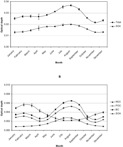
The seasonality of the calculated OD SOA is strong (OD SOA during summer is more than double that of winter; Fig. 10), but the interannual variability is weak (about 12%; not shown) and of the same order of magnitude with the natural variability of

25

(13)

calcu-ACPD

5, 1255–1283, 2005

organic aerosol

Title Page

Tables Figures

◭ ◮

Back Close

Full Screen / Esc

Print Version

EGU

lations that neglect sea-salt and dust, OD SOA contributes to the total global average OD by about 5% with other contributors being sulphate (57%), black carbon (14%), nitrate (13%) and primary organic carbon (11%). These contributions are subject to significant spatial and temporal variations.

6. Conclusions

5

Kanakidou et al. (2000) have shown that the human impact has drastically increased the biogenic SOA chemical production since preindustrial period. This enhanced SOAb chemical production exhibits naturally driven variations that have been studied here. This naturally driven variation in the biogenic SOA production is calculated to equal about 8% i.e. to be of the same order with the chemical production of SOA from

anthro-10

pogenic VOC oxidation, whereas the SOA burden issued from biogenic VOC oxidation varies by about 11.5%.

Meteorological parameters like temperature, water cycle and mixing by transport can affect the temporal and spatial variability of SOA. In particular with regard to the chemi-cal production of SOA from biogenic VOC oxidation, temperature affects the

condensa-15

tion of semivolatile compounds to the aerosol phase, while the water cycle has a major impact by affecting the removal of aerosols from the atmosphere, the water associated to the aerosol and finally the aerosol optical properties. Atmospheric circulation affects the transport of aerosols, which will change the surfaces available for condensation of the semivolatile compounds. According to our calculations this feedback mechanism

20

seems to compensate for the effects of temperature and water cycle changes.

(14)

ACPD

5, 1255–1283, 2005

organic aerosol

Title Page

Tables Figures

◭ ◮

Back Close

Full Screen / Esc

Print Version

EGU

References

Barsanti, K. C. and Pankow, J. F.: Thermodynamics of the formation of atmospheric organic particulate matter by accretion reactions – part 1: aldehydes and ketones, Atmos. Environ., 38, 4371–4382, 2004.

Bonn, B., von Kuhlmann, R., and Lawrence, M. G.: High contribution of biogenic hy-5

droperoxides to secondary organic aerosol formation, Geophys. Res. Lett., 31, L10108, doi:10.1029/2003GL019172, 2004.

Chung, S. H. and Seinfeld, J. H.: Global distribution and climate forcing of carbonaceous aerosols, J. Geophys. Res., 107, 4407–4440, doi:10.1029/2001JD001397, 2002.

Claeys, M., Graham, B., Vas, G., Wang, W., Vermeylen, R., Pashynska, V., Cafmeyer, J., 10

Guyon, P., Andreae, M. O., Artaxo, P., and Maenhaut, W.: Formation of secondary organic aerosols through photooxidation of isoprene, Science, 303, 1173–1176, 2004a.

Claeys, M., Wang, W., Ion, A. C., Kourtchev, I., Gelencs ´er, A., and Maenhaut, W.: Formation of secondary organic aerosols from isoprene and its gas-phase oxidation products through reaction with hydrogen peroxide, Atmos. Environ., 38, 4093–4098, 2004b.

15

de Rosnay, P. and Polcher, J.: Modeling root water uptake in a complex land surface scheme coupled to a GCM, Hydrol. Earth System Sci., 2, 239–256, 1998.

Dentener, F. J., Feichter, J., and Jeuken, A.: Simulation of the transport of Rn222 using on-line and off-line global models at different horizontal resolutions: a detailed comparison with measurements, Tellus, 51B, 573–602, 1999.

20

Derwent, R. G., Collins, W. J., Jenkin, M. E., Johnson, C. E., and Stevenson, D. S.: The global distribution of secondary particulate matter in a 3-D Lagrangian chemistry transport model, J. Atmos. Chem., 44, 57–95, 2003.

Ducoudr ´e, N. I., Laval, K., and Perrier, A.: SECHIBA, a new set of parameterizations of the hydrologic exchanges at the land-atmosphere interface within the LMD atmospheric general 25

circulation model, J. Climate, 6, 248–273, 1993.

Ervens, B., Feingold, G., Frost, G. J., and Kreidenweis, S. M.: A modelling study of aqueous production of dicarboxylic acids, 1: Chemical pathways and organic mass production, J. Geophys. Res., 109, D15205, doi:10.1029/2003JD004387, 2004.

Falkowski, P., Scholes, R. J., Boyle, E., Canadell, J., Canfield, D., Elser, J., Gruber, N., Hib-30

(15)

ACPD

5, 1255–1283, 2005

organic aerosol

Title Page

Tables Figures

◭ ◮

Back Close

Full Screen / Esc

Print Version

EGU

knowledge of earth as a system, Science, 290, 291–296, 2000.

Gibson, R., Kallberg, P., and Uppala, S.: The ECMWF re-analysis (ERA) project, ECMWF newsletter, 73, 7–17, 1997.

Griffin, R. J., Cocker III, D. R., Seinfeld, J. H., and Dabdub, D.: Estimate of global atmospheric organic aerosol from oxidation of biogenic hydrocarbons, Geophys. Res. Lett., 26, 2721– 5

2724, 1999.

Guenther, A., Baugh, B., Brasseur, G., Greenberg, J., Harley, P., Klinger, L., Serc¸a, D., and Vier-ling, L.: Isoprene emission estimates and uncertainties for the Central African EXPRESSO study domain, J. Geophys. Res., 104, 30 625–30 639, 1999.

Guenther, A., Geron, C., Pierce, T., Lamb, B., Harley, P., and Fall, R.: Natural emissions of non-10

methane volatile organic compounds, carbon monoxide, and oxides of nitrogen from North America, Atmos. Environ., 34, 2205–2230, 2000.

Guenther, A., Hewitt, C. N., Erickson, D., Fall, R., Geron, C., Graedel, T., Harley, P., Klinger, L., Lerdau, M., McKay, W. A., Pierce, T., Scholes, B., Steinbrecher, R., Tallamraju, R., Taylor, J., and Zimmerman, P.: A global model of natural volatile organic compound emissions, J. 15

Geophys. Res., 100, 8873–8892, 1995.

Hall, F. G., Collatz, G., Los, S., Brown de Colstoun, E., and Landis, D. (Eds.): ISLSCP Initiative II, DVD/CD-ROM, NASA, 2004.

Herrmann, H.: Kinetics of Aqueous Phase Reactions Relevant for Atmospheric Chemistry, Chem. Rev., 103, 12, 4691–4716, 2003.

20

Houweling, S., Dentener, F., and Lelieveld, J.: The impact of nonmethane hydrocarbon com-pounds on tropospheric chemistry, J. Geophys. Res., 103, 10 673–10 696, 1998.

Janson, R. and De Serves, C.: Acetone and monoterpene emissions from the boreal forest in northern Europe, Atmos. Environ., 35, 4629–4637, 2001.

Jeuken, A., Veefkind, J. P., Dentener, F., Metzger, S., and Gonzalez, C. R.: Simulation of the 25

aerosol optical depth over Europe for August 1997 and a comparison with observations, J. Geophys. Res., 106, 28 295–28 311, 2001.

Kalberer, M., Paulsen, D., Sax, M., Steinbacher, M., Dommen, J., Prevot, A. S. H., Fisseha, R., Weingartner, E., Frankevich, V., Zenobi, R., and Baltensperger, U.: Identification of polymers as major components of atmospheric organic aerosols, Science, 303, 1659–1662, 2004. 30

(16)

ACPD

5, 1255–1283, 2005

organic aerosol

Title Page

Tables Figures

◭ ◮

Back Close

Full Screen / Esc

Print Version

EGU

Vignati, E., Stephanou, E. G., and Wilson, J.: Organic aerosol and global climate modelling: a review, Atmos. Chem. Phys. Discuss., 4, 5855–6024, 2004,

SRef-ID: 1680-7375/acpd/2004-4-5855.

Kanakidou, M., Tsigaridis, K., Dentener, F. J., and Crutzen, P. J.: Human-activity-enhanced formation of organic aerosols by biogenic hydrocarbon oxidation, J. Geophys. Res., 105, 5

9243–9254, 2000.

Kesselmeier, J. and Staudt, M.: Biogenic volatile organic compounds (VOC): An overview on emission, physiology, and ecology, J. Atm. Chem., 33, 23–88, 1999.

Kiehl, J. T. and Briegleb, B. P.: The relative roles of sulfate aerosols and greenhouse gases in climate forcing, Science, 260, 311–314, 1993.

10

Krinner, G., Viovy, N., De Noblet, N., Og ´ee, J., Polcher, J., Friedlingstein, P., Ciais, P., Sitch, S., and Prentice, I. C.: A dynamic global vegetation model for stud-ies of the coupled atmosphere-biosphere system, Glob. Biogeochem. Cyc., 19, 1, doi:10.1029/2003GB002199, 2005.

Kulmala, M., Suni, T., Lehtinen, K. E. J., Dal Maso, M., Boy, M., Reissell, A., Rannik, ¨U., Aalto, 15

P., Keronen, P., Hakola, H., B ¨ack, J., Hoffmann, T., Vesala, T., and Hari, P.: A new feedback mechanism linking forests, aerosols, and climate, Atmos. Chem. Phys., 4, 557–562, 2004, SRef-ID: 1680-7324/acp/2004-4-557.

Lack, D. A., Tie, X. X., Bofinger, N. D., Wiegand, A. N., and Madronich, S.: Seasonal variability of secondary organic aerosol: A global modelling study, J. Geophys. Res., 109, D03203 20

doi:10.1029/2003JD003418, 2004.

Liousse, C., Penner, J. E., Chuang, C., Walton, J. J., Eddleman, H., and Cachier, H.: A global three-dimensional model study of carbonaceous aerosols, J. Geophys. Res., 101, 19 411– 19 432, 1996.

MacDonald, R. and Fall, R.: Detection of substantial emissions of methanol from plants to the 25

atmosphere, Atmos. Environ., 27A, 1709–1713, 1993.

Naik, V., Delire, C., and Wuebbles, D. J.: Sensitivity of biogenic isoprenoid emissions to climate variability and atmospheric CO₂, J. Geophys. Res., 109, doi:10.1029/2003JD004236, 2004. Olivier, J., Bouwman, A. F., Van der Maas, C. W. M., Berdowski, J. J. M., Veldt, C., Bloos, J. P. J.,

Visschedijk, A. J. H., Zandveld, P. Y. J., and Haverlag, J. L.: Description of EDGAR Version 30

2.0: a set of emission inventories of greenhouse gases and ozone depleting substances for all anthropogenic and most natural sources on a per country basis and on 1◦

×1◦ grid, RIVM

(17)

ACPD

5, 1255–1283, 2005

organic aerosol

Title Page

Tables Figures

◭ ◮

Back Close

Full Screen / Esc

Print Version

EGU

Pun, B. K., Wu, S. Y., Seigneur, C., Seinfeld, J. H., Griffin, R. J., and Pandis, S. N.: Uncer-tainties in modelling secondary organic aerosols: Three-dimensional modelling studies in Nashville/West Tennessee, Environ. Sci. Technol., 37, 3647–3661, 2003.

Sitch, S., Smith, B., Prentice, I. C., Arneth, A., Bondeau, A., Cramer, W., Kaplan, J. O., Levis, S., Lucht, W., Sykes, M. T., Thonicke, K., and Venevsky, S.: Evaluation of ecosystem dynamics, 5

plant geography and terrestrial carbon cycling in the LPJ dynamic global vegetation model, Glob. Ch. Biol., 9, 161–185, 2003.

Tegen, I., Hollrig, P., Chin, M., Fung, I., Jacob, D., and Penner, J.: Contribution of different aerosol species to the global aerosol extinction optical thickness: Estimates from model results, J. Geophys. Res., 102, 23 895–23 915, 1997.

10

Tolocka, M. P., Jang, M., Ginter, J., Cox, F., Kamens, R., and Johnston, M.: Formation of oligomers in secondary organic aerosol, Environ. Sci. Technol., 38, 1428–1434, 2004. Tsigaridis, K. and Kanakidou, M.: Global modelling of secondary organic aerosol in the

tropo-sphere: A sensitivity analysis, Atmos. Chem. Phys., 3, 1849–1869, 2003, SRef-ID: 1680-7324/acp/2003-3-1849.

15

Veefkind, P.: Aerosol satellite remote sensing, PhD thesis, Utrecht University, The Netherlands, 1999.

Warneck, P.: In-cloud chemistry opens pathway to the formation of oxalic acid in the marine atmosphere, Atmos. Environ., 37, 2423–2427, 2003.

(18)

ACPD

5, 1255–1283, 2005

organic aerosol

Title Page

Tables Figures

◭ ◮

Back Close

Full Screen / Esc

Print Version

EGU Table 1.Global SOA budget and its variability between 1986 and 1990 due to meteorology and

to changes in biogenic emissions.

Burden Wet deposition Dry deposition Chemical production SOAa SOAb SOAa SOAb SOAa SOAb SOAa SOAb

Gg Gg Tg y−1 _{Tg y}−1 _{Tg y}−1 _{Tg y}−1 _{Tg y}−1 _%a _{Tg y}−1 _%a

M86/E86 12.2 142.9 1.45 17.20 0.11 2.73 1.57 0 20.28 0 T90/E86 12.3 143.8 1.47 17.14 0.11 2.71 1.58 0.6 20.19 −0.4

TH90/E86 16.1 189.1 1.57 17.60 0.11 2.73 1.69 7.6 20.68 2.0 M90/E86 12.5 146.8 1.44 17.83 0.11 2.67 1.56 −0.6 20.26 −0.1

M90/E90 12.5 159.5 1.45 18.67 0.11 2.89 1.56 −0.6 21.94 8.2

a_{% di}

(19)

ACPD

5, 1255–1283, 2005

organic aerosol

Title Page

Tables Figures

◭ ◮

Back Close

Full Screen / Esc

Print Version

EGU Table 2.Extinction coefficients at 555 nm used in the OD calculations.

Aerosol component B(m2g−1₎ _Reference

SO₄ 5 Jeuken et al. (2001)

NO₃ 5 Jeuken et al. (2001)

BC 9 Liousse et al. (1996); Tegen et al. (1997)

Primary OA 4 Liousse et al. (1996)

(20)

ACPD

5, 1255–1283, 2005

organic aerosol

Title Page

Tables Figures

◭ ◮

Back Close

Full Screen / Esc

Print Version

EGU Fig. 1.Difference in temperature (top panels), water vapour (medium panels) and precipitation

(21)

ACPD

5, 1255–1283, 2005

organic aerosol

Title Page

Tables Figures

◭ ◮

Back Close

Full Screen / Esc

Print Version

EGU Fig. 2. Biogenic VOC emissions variability for the period 1984–1993 as calculated by the

(22)

ACPD

5, 1255–1283, 2005

organic aerosol

Title Page

Tables Figures

◭ ◮

Back Close

Full Screen / Esc

Print Version

EGU Fig. 3. Mean terpene emissions for 1986 (top panels) and differences of the mean terpene

(23)

ACPD

5, 1255–1283, 2005

organic aerosol

Title Page

Tables Figures

◭ ◮

Back Close

Full Screen / Esc

Print Version

EGU Fig. 4.Variability of the global annual chemical production of SOA (solid squares), of the SOA

(24)

ACPD

5, 1255–1283, 2005

organic aerosol

Title Page

Tables Figures

◭ ◮

Back Close

Full Screen / Esc

Print Version

EGU

<HDU 1

RU P DO L] HG U DW LR

&KHPLFDOSURGXFWLRQ92&HPLVVLRQVPHDQ H %XUGHQ92&HPLVVLRQVPHDQ

(25)

ACPD

5, 1255–1283, 2005

organic aerosol

Title Page

Tables Figures

◭ ◮

Back Close

Full Screen / Esc

Print Version

EGU Fig. 6. OD SOA for 1986 (top panels) and the difference of OD SOA for 1986 from that for

(26)

ACPD

5, 1255–1283, 2005

organic aerosol

Title Page

Tables Figures

◭ ◮

Back Close

Full Screen / Esc

Print Version

EGU Fig. 7. Tropospheric O₃column (up to 300 hPa, in DU) difference between 1986 and 1990 for

(27)

ACPD

5, 1255–1283, 2005

organic aerosol

Title Page

Tables Figures

◭ ◮

Back Close

Full Screen / Esc

Print Version

EGU Fig. 8.Impact of temperature on OD SOA (top panels) and O₃(bottom panels) for winter (left

(28)

ACPD

5, 1255–1283, 2005

organic aerosol

Title Page

Tables Figures

◭ ◮

Back Close

Full Screen / Esc

Print Version

EGU Fig. 9. Impact of water cycle on OD SOA (top panels) and O₃ (bottom panels) for winter (left

(29)

ACPD

5, 1255–1283, 2005

organic aerosol

Title Page

Tables Figures

◭ ◮

Back Close

Full Screen / Esc

Print Version

EGU !

" #

$ %

&%