i
ANALYSIS OF TEMPORAL AND SPATIAL VARIATION OF FOREST
A case of study in northeastern Armenia
ii ANALYSIS OF TEMPORAL AND SPATIAL VARIATION OF FOREST
A case of study in northeastern Armenia
Dissertation supervised by
Supervisor:
Prof. Dr. Edzer Pebesma, Institute for Geoinformatics, University of Muenster
Co-supervisors:
Prof. Mark Padgham, Institute for Geoinformatics, University of Muenster
Prof. Filiberto Pla, Institute of New Imaging Technologies University Jaume I
iii DECLERATION OF ORIGINALITY
The following Master thesis was prepared in my own words without any additional help. All
used sources of literature are listed at the end of the thesis.
The thesis was not submitted in the same or in a similar version to achieve an academic
grading.
iv ACKNOWLEDGMENTS
I appreciate my supervisor Prof. Dr. Edzer Pebesma for the great support, guidance and
constructive comments. Also I would like to thank co-supervisors Prof. Mark Padgham and
Prof. Filiberto Pla for their time spent on my thesis.
I want to thank Ms. Ana Sousa, Prof. Dr. Marco Pinho, Prof. Brox and to every member of
staff at ifgi and UNL for my wonderful study experience.
I can’t thank enough GEE developers and especially Ian Hausman for continuous support and assistance.
I would especially like to thank Prof. Samvel Nahapetyan and Prof. Hovik Sayadyan for their
help and encouragement.
Last but not the least I would like to thank my family and friends for encouragement, support
v ANALYSIS OF TEMPORAL AND SPATIAL VARIATION OF FOREST
A case of study in northeastern Armenia
ABSTRACT
The forest has a crucial ecological role and the continuous forest loss can cause colossal
effects on the environment. As Armenia is one of the low forest covered countries in the
world, this problem is more critical. Continuous forest disturbances mainly caused by illegal
logging started from the early 1990s had a huge damage on the forest ecosystem by
decreasing the forest productivity and making more areas vulnerable to erosion. Another
aspect of the Armenian forest is the lack of continuous monitoring and absence of accurate
estimation of the level of cuts in some years.
In order to have insight about the forest and the disturbances in the long period of time we
used Landsat TM/ETM + images. Google Earth Engine JavaScript API was used, which is an
online tool enabling the access and analysis of a great amount of satellite imagery.
To overcome the data availability problem caused by the gap in the Landsat series in
1988-1998, extensive cloud cover in the study area and the missing scan lines, we used pixel based
compositing for the temporal window of leaf on vegetation (June-late September).
Subsequently, pixel based linear regression analyses were performed.
Vegetation indices derived from the 10 biannual composites for the years 1984-2014 were
used for trend analysis.
In order to derive the disturbances only in forests, forest cover layer was aggregated and the
original composites were masked. It has been found, that around 23% of forests were
vi TABLE OF CONTENT
DECLARATION OF ORIGINALITY... iii
ACKNOWLEDGMENTS... iv
ABSTRACT... v
TABLE OF CONTENT... vi
KEYWORDS... viii
ACRONYMS... ix
INDEX OF TABLES... x
INDEX OF FIGURES... xi
CHAPTER I INTRODUCTION... 1
1.1. Theoretical Framework... 1
1.2. Statement of the Problem... 3
1.3. Study Area at glance... 4
1.4. Aim and Objectives... 5
1.5. Thesis Organization... 7
CHAPTER 2 CONCEPTS AND DEFINITIONS... 9
2.1. The Use of Remotely Sensed Data for Forest Monitoring... 9
2.2. Forest and Deforestation... 14
2.3. Time Series Analysis... 15
CHAPTER 3 METHODOLOGY... 20
3.1. Workflow... 20
3.2. Study Area... 22
3.3. Materials and Tools... 26
3.4. Research Limitations... 27
CHAPTER 4 DATA PREPARATION... 29
4.1. Image Preprocessing... 29
4.2. The Results of Data Preparation... 32
CHAPTER 5 DETECTION OF FOREST DISTURBANCE AND TREND ANALYSIS... 34
5.1. Image Processing... 34
5.2. Trend Analysis... 35
vii CHAPTER 6
RESULTS AND DISCUSSION... 42
CONCLUSIONS AND RECOMMENDATIONS... 45
BIBLIOGRAPHY... 47
ATTACHMENTS... 51
viii KEYWORDS
Forest
Forest disturbances Trend analysis
ix ACRONYMS
GEE– Google Earth Engine
TM– Thematic mapper
ETM+– Enhanced thematic mapper
VI– Vegetation index
NIR– Near Infrared
SWIR– Short Wave Infrared
NDVI– Normalized Difference Vegetation Index
NDMI –Normalized Difference Moisture Index
ATP – Armenian tree project
FAO– Food and Agriculture Organization of the United Nations
x INDEX OF TABLES
Table 1: The summary of the thesis………. 7
Table 2: The spectral characteristics of Landsat 4-5TM and Landsat 7 ETM+…... 11
xi INDEX OF FIGURES
Figure 1: The volume of forest logging in Armenia derived from available sources
Moreno-Sanchez et al., (2005); Hergnyan et al., (2006); Hayantar (2014)………..…… 4
Figure 2: Wind-fallen trees in Stepanavan……….……….. 5
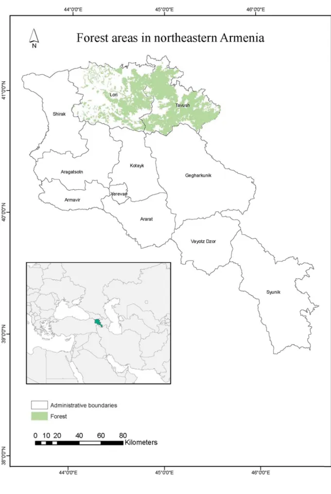
Figure 3: Types of forest in Armenia(Global Forest Watch, Armenia)………….…... 22
Figure 4: Forest loss in the study area (Hansen et al., 2013)……….. 24
Figure 5: Location map of the study area……… 25
Figure 6: Flow chart of preprocessing steps………... 29
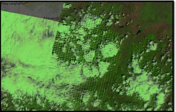
Figure 7: False color composite of Landsat image of year 2003……… 30
Figure 8: False color composite of Landsat image of year 2003 after cloud and shadow masking……… 31
Figure 9: False color composite of Landsat image of year 1985………... 33
Figure 10: False color composite of Landsat image of years 2003-2004……..……….. 33
Figure 11: Long term trends of NDVI (Using FormaTrend) ………..……… 36
Figure 12: Long term trends of NDMI (Using FormaTrend)……….… 36
Figure 13: Long term trends of NDMI (Using linear reducer)……….…….. 37
Figure 14: Long term trends of NDVI (Using linear reducer) ……….……... 37
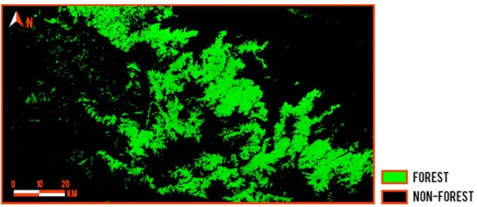
Figure 15: Generated forest cover layer………..………. 39
Figure 16: Forest trends estimated using NDVI……….……. 39
Figure 17: Forest trends estimated using NDMI……….……..………... 40
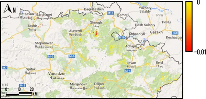
Figure 18: Negative NDMI trends (after non-forest masking)………. 40
Figure 19: Negative NDVI trends (after non-forest masking)………...……….. 41
1
CHAPTER ONE
INTRODUCTION
1.1
Theoretical Framework
Deforestation and forest degradation are one of the biggest environmental problems and their
impact can be colossal. Forests, the most complex terrestrial ecosystems on the earth, have
an important ecological role in the conservation of biological diversity, they store a vast
amount of carbon, prevent soil erosion.
Forest cover changes, especially those of anthropogenic origin, have broad impacts on
critical environmental processes including Earth's energy balance, water cycle, and
biogeochemical processes. Quantifying such changes is required for addressing many
pressing issues including the global carbon budget, ecosystem dynamics, sustainability, and
the vulnerability of natural and human systems (Huang et al., 2008).
Scientists and policy makers from various institutions and agencies are currently devoting
substantial time and resources to study the implications of the environmental change in
forests and woodlands, the most widely distributed ecosystem on earth (Rogan et al., 2006).
Forests provide key ecological goods and services for many other plants and animals, as well
as for humans (Weng, 2011). Consequently, the reduction of the forested area can have
dramatic outcomes. Although the rate of deforestation shows signs of decreasing, it is still
alarmingly high. It shows signs of decreasing in several countries but continues at a high rate
in others (FAO, 2010).
In general, deforestation has been attributed to socio-demographic factors, such as population
growth, economy and specific exploitation activities like commercial logging, forest farming,
fuel wood gathering, and pasture clearance for cattle production (FAO, 2007).
The current state of deforestation is critical in Armenia as well. The Armenian forests are
under the highest socioeconomic pressures, threat of degradation or destruction
(Moreno-Sanchez et al., 2007). This is due to uncontrolled forest logging, which was at its peak
starting from early 1990s. As reported by the Armenian tree project, Armenia is facing one of
the worst ecological threats. In fact, over 750,000 cubic meters of forest coverage are now
being cut annually. At the current rate of deforestation, Armenia faces the probability of
turning into a barren desert within 50 years (Armenian tree project, 2013). Hergnyan et al.,
2 is less than 10% of the total land area. Hence, the continuing deforestation of forest
resources presents a significant environmental threat combined with destroying consequences
for habitats, irreversible losses of biodiversity, lost revenue of the government from the
alternative benefits of the forest (e.g. tourism development). The economic crisis and the
drastic socio-economic conditions, along with the poor implementation of forest management
and monitoring policies throughout the 1990s have resulted in massive deforestation of the
country. Due to the strengthened state control during the recent years the logging volumes
have decreased. However, the overall decrease of the forest resources is still progressing,
despite the major efforts of international and local organizations towards intensive
reforestation. Taking into account economic, social and political conditions in the country,
Moreno-Sanchez et al., (2005) predict that the decline of the forest will continue and it will
probably accelerate.
Because of absence of continuous forest monitoring in the study area, there is a need of
studies which will reveal the current state of forest ecosystems, rate of deforestation,
disturbances during long period and it can give essential contribution in decision making for
sustainable use of forest. To achieve this aim, remotely sensed data can be used.
Remote Sensing provides a unique opportunity to assess and monitor deforestation,
degradation, and fragmentation for a number of reasons. First, it allows detailed study from
local level to global forest resources assessment. Furthermore, remotely sensed data can be
acquired repeatedly (e.g. daily, monthly), which helps to monitor forest resources in a regular
basis (FAO, 2007). Both the gradual changes of forest succession and the sudden change of
deforestation due to anthropogenic (e.g., timber harvesting) or natural (e.g., fire) disturbances
can be detected by satellite imagery. It is usually quite straightforward to map deforestation
with Landsat TM/ETM+ imagery as a result of dramatic change in surface reflectance before
and after the disturbance (Weng 2011).
The increasing availability of satellite imagery with different spatial, spectral and temporal
characteristics and the development of data analysis methods give a chance for having better
idea about forest change patterns. In several studies the potential of detecting changes within
time series is shown, which benefits from temporal depth of satellite imagery and gives an
3
1.2
Statement of the Problem
The last few decades have seen a reduction of the extent and quality of the forest cover in
Armenia. Years of unsustainable and illegal logging have reduced both forest quantity and
quality. Following the independence, an energy crisis led to significant deforestation,
reducing Armenia’s already minimal forest cover.
The decade of the 1990s was harsh and turbulent in Armenia. In 1991 Armenia got its
independence from the former USSR. During the following year the country experienced
political violence and several economic shocks. The separation from the USSR, compounded
by a devastating earthquake in 1988, and the 1988-1994 war with the neighboring Republic
of Azerbaijan created a transportation, economic and energy blockade. This situation put a
tremendous pressure on the forests as source of fuel wood. It is estimated that during the
1990s nearly 50% of the energy consumed in households near to forested areas came from
fuel wood. As a result, the most valuable species of trees were logged (Thuresson et al.,
1999; Moreno-Sanchez et al., 2005; Junge & Fripp 2011).
There is no accurate estimation of the level of cuts during that period and the estimations are
different from author to author. More trustful information about forest logging is available
from late 1990s. Another threat for forest is the copper mining, which occupies large forested
areas in northeastern Armenia.
Figure 1 illustrates the volume of cuts from 1999 till nowadays. The values are aggregated
from different sources (Moreno-Sanchez et al., 2005; Hergnyan et al., 2006; Hayantar 2014),
and they approximate the available data. Although, the economic conditions in the country
have been improved, the volume of cuts remained high for a few years and slowly has been
stabilizing in recent years.
Although there were some studies on forest degradation in Armenia, only few of them have
used geospatial technologies to reveal forest disturbance level. One of the latest studies in
the north-eastern area of Armenia shows the change in forest cover in the study area and
estimates the change from ~25% in 1989 to ~19% in the year 2000 (Asiryan, 2005).
The understanding of seriousness of this problem and the lack of research aiming to detect
the deforestation and the forest degradation and making further analysis were the main
motivation to do this thesis research. Furthermore, the existing studies focus on spatial
change and depict the change from 2 time steps. In this thesis study not only the spatial
4 Figure 1: The volume of forest logging in Armenia derived from available sources
Moreno-Sanchez et al., (2005); Hergnyan et al., (2006); Hayantar (2014)
1.3
Study Area at glance
The study area is located in the north-eastern part of Armenia. The area comprises the biggest
forested areas in Armenia. At the same time this area is described as one of the most
vulnerable areas to deforestation and forest degradation.
The main deforestation threats are fuel wood gathering, infrastructure and mining.
Deforestation in this area is expressed as clear cuts around the large cities. Another major
feature of deforestation process is the accelerated rates of forest fragmentation. The
increasingly complex shapes of large forest patches distort the forestry estimates: the forest
degradation continues leaving the surface of forest cover relatively unchanged (Hergnyan et
al., 2006). In addition to anthropogenic disturbances, large areas of forests are destroyed by
natural causes: wind, erosion and landslides, forest fires. Large areas of forest disturbances
caused by wind were reported in 2004 and 2007 (Hayantar, 2014). Figure 2 illustrates wind
fallen trees in 2007. 0
10000 20000 30000 40000 50000 60000 70000 80000 90000 100000 110000 120000
2000 2001 2002 2003 2004 2005 2006 2007 2008 2009 2010 2011 2012 2013
Volume
of
cuts
The stu
challeng
1.4
Ai
This stu present) differen T o T T The hyp
udy area is
ge for study
ms and O
udy aims at
) based on
nt methods.
To study if
of forest in
To obtain te
To define fo
potheses tha s characteri ying defores Fi (H
Objectives
t detection o
Landsat da Achieving t available L study area emporal tren forest chang
at we yield f
ized by str
station from
igure 2: Wind
Hayantar, 201
s
of the fores
ata. The aim
these aims e
Landsat data
nd
e spatially
from the ab
rong topogr
m remote sen
d-fallen trees
14 http://www
st cover cha
m of the stu
entails the f
a are sufficie
bove mentio
raphy. Its
nsing image
s in Stepanav
w.hayantar.a
ange during
udy is also
following ob
ent for ana
oned objectiv
regular clo
ery.
an
am)
a long per
to assess th
bjectives:
alyzing the p
ves are as fo
oud cover p
riod of time
6 1. With the use of Landsat data forest cover change analysis and trend detection can be
performed.
2. There is a distinct negative trend in forest cover change.
In order to achieve the above mentioned research goals and objectives, the following research
questions need to be reflected on:
Is it possible to detect patterns and trends of forest changes in local scale using
temporally dense Landsat collections? How scientifically robust is the use of those data
to identify the changes in the study area taking into account the limitations of study?
What kind of techniques could be used to analyze forest cover change? Are those methods relevant for research in local scale?
7
1.5
Thesis Organization
Table 1: The summary of the thesis
Is it possible to detect patterns and trends of forest changes in local scale using temporally dense Landsat collections?
PROBLEM
Hypothesis1
With the use of Landsat data forest cover change analysis and trend
detection can be performed
Hypothesis2
There is a distinct negative trend in forest cover change
HYPOT
HESES
Theoreticalstudy:
‐ Literature
‐ Reading and information gathering ‐ Definition of concepts
Empiricalstudy:
‐ Case Study
‐ Performing analysis in Google Earth Engine
‐ Validation
VERIFICATI
ON
Developingthetheoreticalbackgroundwhichwillbethebasisforthe study
THEORETICAL
GOAL
Implementingthealgorithminordertofindtheforestdisturbances duringthestudyperiod
PRACTICAL
8 Table 1 sum up the key points of the thesis. To achieve previously discussed goals and
objectives the master thesis consists of six chapters:
Chapter 1: Introduction
Chapter 1 includes the background and the research problem. It comprises the objectives of
the study, research questions and gives an idea about the study area.
Chapter 2: Concepts and definitions
Chapter two refers the description of general concepts and definitions that are essential for
this research. Furthermore extensive literature review is included, which gives detailed
information about the related studies.
Chapter 3: Methodology
Chapter three contains the main methodological approaches and steps that are followed for
achieving previously discussed goals. It gives detailed description of study area as well as the
data that are used for study. The description of tools and programming environment is also
included. The study limitations and constraints are also described in this chapter.
Chapter 4: Data preparation
Chapter four comprises the descriptions of steps of remotely sensed data preprocessing and
preparation.
Chapter 5: Detection of forest disturbance and trend analysis
In chapter five the steps of forest change detection and temporal trend analyses are described.
There is a detailed description of the vegetation indices that have been used. Afterwards the
main steps of implementation of linear regression model and the assessment of the analysis
are described.
Chapter 6: Results and discussion
Chapter six summarizes research findings. Main advantages and disadvantages of used
9
CHAPTER TWO
CONCEPTS AND DEFINITIONS
2.1 The Use of remotely Sensed Data for Forest Monitoring
Various studies have been undertaken in the area of land use and land cover change analysis
and particularly for forest change analysis with the use of remotely sensed data. Relating the
spectral changes among multi temporal satellite data sets to changes in surface features and
biophysical variables has long been an important application of remote sensing technology
(Hayes & Cohen, 2007). The increasing availability of remotely sensed data and the
improvement of data resolution make it even more useful for forest monitoring.
In general, ecosystems can be described by their condition (their state) and by how they are
changing (their temporal dynamics). Remotely sensed data can be successfully used for both
purposes across the number of ecosystem types, including forest (Cohen et al., 2004). Forest
change mapping and monitoring is feasible when changes in the forest attributes of interest
result in detectable changes in image radiance, emitance, or microwave backscatter values
(Rogan et al., 2006). Furthermore, the consistent and objective nature of remote sensing
measurements allows unbiased comparison of forest disturbances (Griffiths et al., 2012).
Several methods were developed for this aim: manual interpretation, algebraic methods
(image differencing, image regression, image ratioing, vegetation index differencing),
transformations, thematic classification, post classification change detection, with the use of
remotely sensed data from variety of sensors as different states of the land surface can be
measured by satellite-derived biophysical parameters (Rogan et al., 2006; FAO 2007; Forkel
et al., 2013).
Change detection approaches can be categorized into two broad groups: bi-temporal change
detection and temporal trajectory analysis. Almost all classifications for change detection
algorithms are based on bi-temporal change detection and little care for temporal trajectory
analysis. For bi-temporal images, any kind of change detection algorithm can be attributed to
one of the following methods: directly compare different data sources, compare extracted
information and detect changes by bringing all the data sources into a uniform model.
Temporal trajectory analysis can be decomposed into bi-temporal change detection and long
time-series analysis(Jianya et al., 2008).
The most common approaches used in change detection have included the post classification
10 differencing of single bands or band ratios. Multivariate techniques that incorporate more
spectral information in the change detection algorithm often produce improved results.
Examples include clustering of multi temporal composite images and the use of multivariate
transformations such as the tasseled cap, principal components analysis and the less used
canonical correlation analysis (Hayes & Cohen, 2007).
In their study Hirschmugl et al., (2014) describe the methods that can be used for mapping
forest degradation from optical data: simple spectral band values, vegetation indices,
proximity to new roads (context analysis), or more advanced tools, such as spectral mixture
analysis and related indices, such as the Normalized Difference Fraction Index, or different
combinations of these features.
An important issue for forest change detection and analysis is the selection of satellite
imagery. The choice of the imagery depends on many factors such as the objectives of the
research, characteristics of study area, spatio-temporal resolution of imagery and the costs. If
the study is focused on temporal trajectory analysis, forest change analysis is mostly based on
low spatial resolution images such as AVHRR and MODIS, which have a high temporal
resolution (Jianya et al., 2008).
Another widely used data for forest change analysis is Landsat imagery. The spatial
resolution of imagery is informative of human activities on the Earth surface and it has made
Landsat invaluable information source for science, management and policy development
(Wulder et al., 2011). Forest change detection with Landsat has a history as long as the
Landsat program itself (Cohen et al., 2010). The 30 m pixel size of the Landsat TM and
ETM+ sensors makes them suitable to characterize the land-cover change resulting from
natural and anthropogenic activities.
The number and placement of spectral bands is also an important advantage over other similar
sensors and the spectral information of vegetation in Landsat TM and ETM+ imagery is
primarily determined by the designation of spectral bands as seen in Table 2. The Thematic
mapper (TM) and Enhanced thematic mapper (ETM+) sensors acquire the images in visible,
near infrared and shortwave infrared portions of the electromagnetic spectrum, making them
appropriate for studies of vegetation properties across a wide range of vegetation
communities, in diverse environments (Bhandari et al., 2012). In Table 2 the spectral
characteristics of Landsat TM and ETM+ are described (Landsat missions, USGS, 2014). In
the first three bands, reflected energy from vegetation is determined by the concentration of
leaf pigment. Leaves strongly absorb solar radiation in the visible spectrum, particularly the
11 spectrum, to which healthy green leaves are highly reflective. In fact, the contrast in leaf
reflectance between the red and NIR spectra is a physical basis for numerous vegetation
indices using optical remote sensing. The two mid-infrared bands relate to the moisture
content in healthy vegetation (Weng, 2011). These two bands are also very sensitive to
vegetation density, especially in the early stages of clear cut regeneration.
Table 2: The spectral characteristics of Landsat 4-5 Thematic Mapper (TM) and Landsat 7 Enhanced
Thematic Mapper Plus (ETM+)
Band Wavelength Useful for mapping
Band 1 - blue 0.45-0.52 Bathymetric mapping, distinguishing soil from vegetation and deciduous from coniferous vegetation
Band 2 - green 0.52-0.60 Emphasizes peak vegetation, which is useful for assessing plant vigor
Band 3 - red 0.63-0.69 Discriminates vegetation slopes
Band 4 - Near Infrared 0.77-0.90 Emphasizes biomass content and shorelines
Band 5 - Short-wave Infrared
1.55-1.75 Discriminates moisture content of soil and vegetation; penetrates thin clouds
Band 6 - Thermal Infrared
10.40-12.50 Thermal mapping and estimated soil moisture
Band 7 - Short-wave Infrared
2.09-2.35 Hydrothermally altered rocks associated with mineral deposits
Band 8 - Panchromatic (Landsat 7 only)
.52-.90 15 meter resolution, sharper image definition
Recent studies (Vogelmann et al., 2012; Verbesselt et al., 2012) introduces to four general
categories of vegetative changes, which can be monitored using remotely sensed data:
abrupt change seasonal change
gradual ecosystem change
12 All four types of changes can alter vegetative spectral properties, and depending on the goals
of the investigation, can necessitate the use of different approaches and ancillary data to map
them effectively.
Abrupt changes are the result of changes caused by landscape transforming disturbance
events, such as those related to logging, deforestation, agricultural expansion, urbanization,
and fire. In general, these types of events radically alter the spectral properties of the land
surface, and are readily discernible in Landsat imagery.
Seasonal change relates to the cyclical intra- and inter-annual patterns of phenology, whereby
seasonality influences vegetation condition in predictable and mostly repeatable patterns of
green-up and senescence. Similar to abrupt change, phenological change can have marked
impacts on spectral characteristics of the vegetation, and tend to be especially pronounced in
deciduous forest.
Gradual ecosystem change relates to subtle within-state changes taking place in vegetation
communities that are not related to normal phenological cycles. These include a variety of
within state disturbances, such as vegetation damage caused by insects and disease, drought
and storms, changes in plant communities related to natural succession, grazing pressure, and
climate-induced biome shifts.
The last group of changes is short-term inconsequential vegetative change which is a number
of events that cause vegetative spectral changes not perceived as having long-term ecological
importance. These include rain-fall events that affect spectral properties of the soil
background wind that affects leaf angles during the time of data acquisition), and light frost
or snow on conifer vegetation at high elevations, occurring especially during the beginning
and end of the growing season. These events may be considered as noise by most analysts as
they can have marked impacts on the spectral properties of the data sets being analyzed,
which can in turn alter interpretations and create a level of uncertainty in remotely sensed
data sets and derived change products. These types of changes tend to be difficult to
characterize, and are largely ignored in most change investigations.
Another change that is taking place in forest areas is forest growth which is always a gradual
process. Establishment of forest stand always takes time, and trees continue to grow after the
stand is established (Weng, 2011).
Vogelmann et al., (2012) discuss the use of Landsat imagery for forest change analysis and
they depict that Landsat imagery is applicable for detecting abrupt and gradual ecosystem
13 difficulty in acquiring enough quality cloud-free data sets to adequately characterize the
phenological variability within an ecosystem. Nevertheless, Landsat data provide useful
complementary data when used in conjunction with the high temporal resolution data in
phenological assessments.
With few exceptions, most research with the use of Landsat imagery have focused on 3–10
years or greater image intervals and one or two Landsat scenes (Cohen et al., 2010). Similar
research was also done for north eastern Armenia. Asiryan (2005) shows data analysis for the
purposes of forest cover change detection for the surrounding areas of Vanadzor city
(north-east Armenia). Two satellite images (Landsat TM/1989 and Landsat ETM+/2000) were
processed and analyzed. The results indicated that a significant change in land cover occurred
between the 1989 and the 2000. In particular, the analysis revealed the reduction of
vegetative cover in the study area.
But as it was shown by Verbesselt et al., (2010), conventional bi-temporal change analysis is
not sufficient as most of the methods focus on short image time series. The risk of
confounding variability with change is high with infrequent images, since disturbances can
occur in between image acquisitions. Similar study clearly highlights the considerable
advantages that the annual temporal resolution of the Landsat time series holds over bi- or
multi temporal change detection approaches. For example, a change map at five or 10-year
interval would not have been able to distinguish a large disturbance occurring in a single year
from individual patches clustering to a large area over time (Griffiths et al., 2012).
In addition, although many disturbances often result in abrupt spectral changes that are
relatively easy to detect using satellite images acquired before and immediately after each
disturbance, the spectral change signals often become obscured and eventually undetectable
as trees grow back following those disturbances. As a result, forest change products derived
using temporally sparse observations typically have considerable omission error (Weng,
2011). In another study of Verbesselt et al., (2012) was described that detecting changes
within time series is the step towards understanding the acting processes and drivers (e.g.,
natural or anthropogenic). The detailed use of this method is described in the following
14
2.2 Forest and Deforestation
Before studying the techniques for analyzing spatial and temporal variations of forest, it is
important to distinguish the main concepts regarding forest degradation and deforestation.
There are many definitions and here some of them are described which gives better insight
and understanding of those processes.
1. Forest: Moreno-Sanchez et al., (2007) define the terms forest cover or forest to denote high forests (natural or created by plantations) dominated by tree species. The
definition of forest is critical for this study as it defines the area where the changes are
estimated.
2. Forest change: In the context of environmental remote sensing, forest change, manifested as forest attribute modification or conversion, can occur at every temporal and
spatial scale, and changes at local scales can have cumulative impacts at broader scales
(Rogan et al., 2006).
FAO (2007) specifies the differences of deforestation and forest degradation, which are
another crucial terms.
3. Deforestation: The conversion of forested areas to non-forest land use such as arable land, urban use, logged area or wasteland. According to Food and Agriculture Organization
of the United Nations (FAO), deforestation is the conversion of forest to another land use or
the long-term reduction of tree canopy cover below the 10% threshold. Deforestation defined
broadly can include not only conversion to non-forest, but also degradation that reduces
forest quality - the density and structure of the trees, the ecological services supplied, the
biomass of plants and animals, the species diversity and the genetic diversity. Narrow
definition of deforestation is: the removal of forest cover to an extent that allows for
alternative land use.
4. Forest degradation: The process leading to a temporary or permanent deterioration in the density or structure of vegetation cover or its species composition. It is a change in
forest attributes that leads to a lower productive capacity caused by an increase in
disturbances. The time-scale of processes of forest degradation is in the order of a few years
to a few decades. In another study forest degradation was described as a reduction in the
natural or desirable characteristics of a forest (e.g. age, classes, structure, density, or standing
stock genetic quality) (Moreno-Sanchez et al., 2005). Taking into account the specialties of
the study area and particular forest variations, this study is focused on detection of
15 5. Reforestation: Re-establishment of forest formations after a temporary condition with less than 10% canopy cover due to human-induced or natural perturbations. The
definition of forest clearly states that forests under regeneration are considered as forests
even if the canopy cover is temporarily below 10%. Many forest management regimes
include clear-cutting followed by regeneration, and several natural processes, notably forest
fires and windfalls, may lead to a temporary situation with less than 10 percent canopy cover.
In these cases, the area is considered as forest, provided that the re-establishment (i.e.
reforestation) to above 10 percent canopy cover takes place within the relatively near future.
As for deforestation, the time frame is central. The concept temporary is central in this
definition and is defined as less than ten years.
2.3 Time Series Analysis
The recent opening of the global Landsat archive by the United States Geological Survey
(USGS) provides new opportunities to advance land use science and has sparked the
development of new methodological approaches. For example, change detection methods
based on annual Landsat time series (i.e. trajectory-based change detection methods) make
better use of the temporal depth of the Landsat archive to reconstruct forest disturbance
histories with annual resolution and to map trends, such as forest regeneration and
succession. Likewise, annual time series of Landsat images can help to separate sudden from
gradual vegetation change (Griffiths et al., 2012). Cohen et al., (2010), mentions about
tremendous need for temporally and spatially detailed forest change information over vast
areas for forest management and policy considerations.
Estimating change from remotely sensed data series however is not straightforward, since
time series contain a combination of seasonal, gradual and abrupt ecosystem changes
occurring in parallel, in addition to noise that originates from the sensing environment (e.g.,
view angle), remnant geometric errors, atmospheric scatter and cloud (Verbesselt et al.,
2012).
One of the algorithms is a trajectory based change detection algorithm developed by Kennedy
et al., (2007). The main premise of the method is the recognition that many phenomena
associated with changes in land cover have distinctive temporal progressions both before and
after the change event, and that these lead to characteristic temporal signatures in spectral
space. Rather than search for single change events between two dates of imagery, they instead
searched for idealized signatures in the entire temporal trajectory of spectral values. If an area
16 is likely to have experienced the phenomenon described by that trajectory. Because the entire
trajectory was considered, the method utilized the depth of rich image archives, and because
detection was based on the fit of a curve, thresholds were based on a statistical metric that is
internally calibrated to each pixel, avoiding the need for manual interpretation or intervention.
Another study shows validation of North American forest disturbance dynamics derived from
Landsat time series stacks with biennial time steps. For further analysis they use vegetation
change tracker (VCT) algorithm specifically for mapping forest change using Landsat time
series stuck or data sets that consist of temporally dense satellite acquisition. The algorithm
consists of two major steps: 1) individual image analysis and 2) time series analysis (Thomas
et al., 2011).
Griffiths et al., (2012) discuss, that the analysis of an annual Landsat time series with
trajectory-based change detection methods (such as LandTrendr) can provide deep insight
into the effects of the institutional and socioeconomic changes on forests.
Another complex approach is proposed for automated change detection in time series by
detecting and characterizing Breaks For Additive Seasonal and Trend (BFAST) by Verbesselt
et al., (2010). BFAST integrates the decomposition of time series into trend, seasonal, and
remainder components with methods for detecting significant change within time series.
BFAST iteratively estimates the time and number of changes, and characterizes change by its
magnitude and direction. They tested BFAST by simulating 16-day composites of Normalized
Difference Vegetation Index (NDVI) time series with varying amounts of seasonality and
noise, and by adding abrupt changes at different times and magnitudes. This revealed that
BFAST can robustly detect change with different magnitudes (>0.1 NDVI) within time series
with different noise levels (0.01–0.07 σ) and seasonal amplitudes (0.1–0.5 NDVI) (Verbesselt et al., 2010).
In several studies (Jin & Sader, 2005; Cohen et al., 2010; Verbesselt et al., 2012, Vogelmann
et al., 2012; Forkel et al., 2013), trends in forest area were analyzed through image-derived
vegetation index and transformations.
Forest disturbances and their subsequent regeneration are often detected and mapped using
spectral indices. These indices are mostly based on the short wave infrared (SWIR) and near
infrared (NIR) reflectance, although forest disturbances can also be detected in the visible or
thermal spectrums. NIR reflectance decreases with an elevated defoliation level and/or after
forest dieback, because bark and soil reflectance is lower than the reflectance of needles or
leaves. Disturbance detection may be complicated when the understory vegetation is not
17 compensate for the decrease in NIR reflectance resulting from forest disturbance. In contrast,
the SWIR reflectance of forest stands is lower than that of the bark, soil, and understory, so
SWIR reflectance increases after forest disturbance (Hais et al., 2009).
Literature is replete with the most frequently used approach for detecting temporal trends:
fitting linear regressions of a (temporally aggregated) vegetation index (VI) against time
(Jong & Bruin, 2012). Vogelmann et al., (2012) describe the use of linear regression
relationships on a pixel by pixel basis between time (x variable) and the vegetation index
value (y variable) for selected pixels. They delineate that regression models with low slope
value tend to not be statistically significant (no apparent change), whereas the models with
high positive or negative slope values are more likely to be statistically significant. Results
from this study indicate that analyses of Landsat time series data provide useful perspectives
regarding long-term gradual ecosystem changes taking place across landscapes. All
investigated areas showed evidence of significant trends in spectral change associated with
the gradual loss and accrual of vegetation canopy cover.
Change detection, however, is often complicated by a number of statistical preconditions that
are intrinsic to time series of spectral vegetation indices with dense sampling intervals, but
this needs to be done with care in order to avoid spurious trends. The detected slope can be
used to calculate the amount of change, but it is not always tested for significant deviation
from zero, nor standard statistical assumptions always respected. Seasonal variation is an
important cause for the data to violate assumptions like homogeneous variation and absence
of serial correlation in the residuals. In few cases linear models were fitted directly to seasonal
data, but seasonality is typically remediated using temporal aggregation, where the
aggregation window corresponds to the length of a calendar year.
Large variation in detected changes was found for aggregation over bins that mismatched full
lengths of vegetative cycles, which demonstrates that aperiodicity in the data may influence
model results. Using VI data and aggregation over full-length periods, deviations in VI gains
of less than 1% were found for annual periods (with respect to seasonally adjusted data),
while deviations increased up to 24% for aggregation windows of 5 year. This demonstrates
that temporal aggregation needs to be carried out with care in order to avoid spurious model
results.
The risk of artefacts is minimal at an aggregation level corresponding to a full period, for
instance a calendar year. Coarser aggregation levels tend to overestimate the amount of
change and result in higher variation in model predictions, especially from 3 periods onwards.
18 hardly ever free of changes in seasonality. Aperiodicity within long-term time series of
vegetation indices is intrinsic to certain land cover types and may arise from variations in start
and length of growing seasons as a result of variations in temperature and/or precipitation
(Jong & Bruin, 2012).
In a latest study of Hansen et al., (2013) it was shown the use of time-series analysis of
654,178 Landsat 7 ETM+ images in characterizing global forest extent and change from 2000
through 2012. As a result tree cover, forest loss, and forest gain was shown during the study
period. Percent tree cover, forest loss and forest gain training data were related to the time
series metrics using a decision tree. Forest loss was disaggregated to annual time scales using
a set of heuristics derived from the maximum annual decline in percent tree cover and the
maximum annual decline in minimum growing season NDVI. Trends in annual forest loss
were derived using an ordinary least squares slope of the regression of annual loss versus
year. This study has significant role in forest change analysis because it has global coverage
and the results can serve for validation of the current study.
Given the limited availability of cloudfree Landsat data in some areas of the globe, epochal
composites have been used extensively to support change detection studies. These
composites represent a new paradigm in remote sensing that is no longer reliant on scene‐
based analysis (White et al., 2014).
A time series of these image composites affords novel opportunities to generate information
products characterizing land cover, land cover change, and forest structural attributes in a
manner that is dynamic, transparent, systematic, repeatable, and spatially exhaustive.
White et al., (2014) proposes three unique types of pixel‐based image composites: annual (single‐year) composites,
multi‐year composites, proxy‐value composites.
Annual composites are surface reflectance composites that use the best available pixel
observation (from the target year) for any given pixel location. Annual composites are
produced using a set of specified rules that are defined according to the information need. For
example, an annual composite may be designed to capture a specific time period or a limited
phenological window. In addition to a day‐of‐year rule, rules may also constrain observations
according to sensor, distance to cloud and cloud shadows, and atmospheric opacity (to reduce
the impact of haze). If there are no observations that satisfy the compositing rules for a given
pixel location, then the pixel is coded as "no data" and as a result, annual composites may
19 Multi‐year composites are generated according to a set of user‐specified rules; however, pixel
observations from previous or subsequent years may be used when no suitable observation is
found within a desired target year.
Proxy value composites are annual composites where no data pixels are populated using a
time series of annual composites to determine proxy values. Likewise, pixels with anomalous
values those that exceed a pre‐defined range of expectation or which have opacity values
indicative of hazy imagery may also be assigned a proxy value. In essence, the objective of
the proxy value composite is to assign the most similar value in time and space to a pixel that
20
CHAPTER THREE
METHODOLOGY
3.1 Workflow
From the review of other researches in the preceding chapter, it is logical to deduce that
temporally dense satellite data can give better idea about trend in forest dynamics.
Based on related studies the main steps of research were developed:
Data preparation and image preprocessing Image processing
Detection and analysis of long term trend
Evaluation of spatial distribution of forest change Validation of results
The goal of preprocessing is to ensure that each pixel faithfully records the same type of
measurement at the same geographic location over the time. Preprocessing is especially
critical in change studies because the detection of change assumes that the spectral properties
of non-changed areas are stable, and inadequate pre-processing can increase error by causing
false change in spectral space (D. Lu & Q. Weng, 2007). This step includes radiometric
corrections and cloud and shadow masking.
Several studies have shown the impact of clouds and cloud shadows on vegetation change
analysis. The pixels contaminated with cloud and shadow generally have sufficiently
different reflectance properties than the actual land cover and produce erroneous information
if used in an automated mapping algorithm (Bhandari et al., 2012). To eliminate this effect
cloud masking function is implemented over the image collection.
The data preparation step also includes the creation of image composites. Characteristics
relevant to particular geographic regions, such as persistence of cloud cover, topography,
dynamism of landscape processes, phenology, and Landsat data availability, are important
considerations when applying a compositing approach. Likewise, different information needs
(e.g., disturbance mapping, estimation of biophysical parameters) may dictate different
compositing strategies, target dates, and compositing rules that are specific to the application.
In general, it is desirable to generate composites that have consistent phenology with minimal
no data pixels that best represent the phenomenon of interest (e.g., land cover classes, forest
21 Pixel‐based image compositing of Landsat data has emerged from a unique confluence of
scientific and operational developments, predicated by free and open access to the Landsat
archive, and supported by computing and data storage capacity to fully automate radiometric
and geometric pre‐ processing and create increasingly robust standardized image products
(White et al., 2014).
Many studies, like Cohen et al., (2010) stated, that the use of dense (nearly annual) Landsat
time series allows characterization of vegetation change over large areas at an annual time
step and at the spatial grain of anthropogenic disturbance. Additionally, it is more accurate in
detection of subtle disturbances and improved characterization in terms of both timing and
intensity. Based on this, time series of Landsat images will be created. It is worth to
mention, that timing and the variation of vegetation phenology should be considered and as a
result, the images should be chosen from the same time of the year and particularly from
peak growing season (early June to late September). It is stated that images acquired outside
this temporal window are generally not suitable for forest change analysis, because leaf off
deciduous forests can be spectrally confused with disturbed forest land. (Weng, 2011).
Time series of vegetation indices (VI) derived from satellite imagery provide a consistent
monitoring system for terrestrial plant productivity. They enable detection and quantification
of gradual changes within the time frame covered. The dependent variable Y can be any kind
of VI or cyclical environmental parameter in general. (Jong & Bruin, 2012).
For this study we used the NDVI, which is a commonly used proxy for terrestrial
photosynthetic activity. To detect the partial harvests with better accuracy NDMI is also
used. The following step is temporal trend analysis. Time series analysis of the rate of change
of forest area is calculated using the slope estimate from linear regression. The slope
indicates the strength of a trend in the change of forest. (Google Earth Engine API tutorial,
2014).
The spatial patterns and the distribution of forest change can be studied by using the results
from image processing step. Afterwards the results are validated by comparing with ground
truth forest harvest data and the data from yearly reports of annual reports of State forest
3.2 Stu
The stu located al., 2005 from 25 preservi MorenoThe te
located Asian, biodiver included compos compos
beech F
et al., 20
Today t
with low forest ty The nor have th Most A
udy Area
udy area is l
in southwe 5). Armenia 50-300 mm ing favorab o-Sanchez, 2 errain comp
at the cros
Iran-Turan
rsity and h
d in the C
sed of 110
sed of comp
Fagus orien
007).
the Armeni
w density,
ypes in Arm
Fig
rth-eastern a
he most fav
Armenian for
located in t
est Asia. Th
a is situated
to 1 000 m
ble environm
2006).
plexity and
sroads of fo
nian and C
high percen
Caucasus an
tree and
plex mixes o
talis, and h
ian forests
low annual
menia.
gure 3: Types http:/
and south-e
vorable clim
rests are fou 5%
he north-ea
he country h
d in a dry su
mm. In this
mental con
microclim
four differen
Caucasian),
ntages of p
nd Irano-An
152 bush s
of broadlea
ornbeam Ca
can be cha
l growth ra
s of forest in A //www.global
eastern parts
matic and en
und in mou %
8%
astern part o
has a total
ubtropical cl
dry-subtrop
nditions for
matic diversi
nt floristic p
produce
plant and an
natolian bi
species. Th
af deciduous
Carpinusbet
aracterized
ates, and po
Armenia (Glo lforestwatch.
s of the cou
nvironment
untainous ter 87%
of Armenia
area of 29
limatic zone
pical region
r sustainabl
ity, as well
provinces (
different v
nimal ende
odiversity
he Armenia
s tree speci
tulus and C.
as overstoc
oor regener
obal Forest W org/country/A
untry and th
tal conditio
rrain betwe
. The Repu
800 km2 (M
e. Annual p
n, forests pl
e developm
l as the fac
Old-Medite
vegetation
emism. Tod
hotspots. T
an forests a
es (mostly
orientalis)
cked and o
ration. Figu
Watch, Armen ARM)
he eastern ba
ons for the
en 500 and Primary
Regenerated
Planted
ublic of Arm
Moreno-San
precipitation
lay a major
ment (Sayad
ct that Arm
erranean, N
types wit
day the cou
The dendro
are predom
Oak Querc
) (Moreno-S
over-mature
ure 3 repres
enia,
ank of Lake
growth of
d 2200 m ab
22 menia is
nchez et
n ranges
r role in
dyan & menia is ear-east th high untry is flora is minantly
us spp.,
23 level. The forest cover is highly fragmented. The 62% of the forest cover is found in the
northeast (Moreno-Sanchez et al. 2005). This was the primary reason of the study area
choice, due to the fact that forests are mostly located in this part of the country, and as stated
by Asiryan, (2005) this areas have suffered damage made over the last twenty years.
The transformations and current state of the Armenian forests result from decades of
management policies and forest use practices by several stakeholders and economic
activities. Planned industrial production or use of the forests was very limited during the
Soviet and independence periods (Moreno-Sanchez et al., 2007). The pressure on forest as a
source of fuel abruptly increased after the independence due to economic blockage. Starting
from these years the forest logging was uncontrolled. There was an attempt by authorities to
control the forest harvest in order to lower the damage caused by cuts. To do so plans were
made to supply fuel wood to the population during 1993. Before 1993, the fuel wood cut was
fixed at 60 000 m3 per year. As a result, in 1993 the harvest was raised to 100 000 m3. In
reality, this plan was difficult to realize because of fuel limitations, and the transportation of
the wood to distribution areas was a major impediment. Estimates of the volume of the illegal
cutting suggest that 700 000-1 000 000 m3 of wood were cut illegally in each of three winters
1992-1995 (Sayadyan, 2007).
Thurresson et al., 1999 stated that forested areas close to population centers became the
main source of fuel wood during the winters of 1991-1993 and were heavily damaged. Legal
and illegal cuttings during 1991-1996 are estimated around 600 000 m3 per year.
Illegal logging in Armenia is conducted mainly by local communities for survival through
unauthorized timber extraction from the state forests. The timber consumed by rural
households was estimated to be 568 000 solid m3 annually. The overall timber production
was estimated 847 000 solid m3 in 2003, from which officially allowed and registered
volume constituted 63 000 m3. Thus cuttings in average is 1 000 000 m3/year, which makes
13 000 000-14 000 000 m3 for last 13-14 years (Sayadyan, 2007).
According to “Hayantar” organization of the Ministry of Agriculture of the Republic of
Armenia, which is the main organization responsible for conservation, protection,
reproduction, use, registration and sustainable use of forest resources, currently there are 19
forest units. For research, 9 forest units and 1 national park were chosen. The 9 forest units
are Ijevan (20955.8 ha), Dsegh (14505.2 ha), Gugarq (10496.9 ha), Sevqar (18236.5 ha),
Arcvaberd (38664.2ha), Noyemberyan (27001 ha), Lalvar (24339.5ha), Jiliza (13851.1ha),
Tashir (5105.2 ha) and Dilijan national park (24000 ha) with more than 190 000 ha (1900
24 Armenia’s forest cover. Also this area is described as one of the most vulnerable to
degradation. Figure 5 illustrates the location of study area in Armenia.
Figure 4: Forest loss in the study area (Hansen et al., 2013)
Figure 4 approximates the forest loss evaluated by Hansen et al., (2013). The data were
accessed directly in GEE and tree loss per year was computed for the area of interest. All the
other numbers and estimates are covering the forest loss in the overall area of Armenia.
Those estimates are relevant, as the most of the forests are located in northeast. Figure 4
provides additional insight about forest dynamics specifically in the study area. It is worth
mentioning that forest loss evaluated by Hansen et al., (2013) have depicted considerably
small value of loss in 2001-2012 (the small values can be accounted for by the global
algorithm) but still it can give an idea about the trends and fluctuations of forest loss in
northeastern Armenia. 0
0,5 1 1,5 2 2,5 3 3,5 4 4,5 5
2001 2002 2003 2004 2005 2006 2007 2008 2009 2010 2011 2012
Forest
loss
Figurre 5: Locattion map off the study area
26
3.3 Materials and Tools
For the study Landsat image collections are used. Data are accessed form Google’s public
catalog, which contains a large amount of publicly available georeferenced imagery,
including most of the Landsat archive (Google Earth Engine. API tutorial, 2014).
For study two image collections are chosen from Landsat TM and ETM+ sensors. Table 3
presents the main parameters of image collections. It should be stressed that data availability
is presented for whole collection and imagery can be unavailable for specific regions and
time period. As far as this study area is concerned, the data are missing for several years.
The choice of Landsat is conditioned by several advantages. First, mission continuity:
Landsat offers the longest-running time series of systematically collected remote sensing
data. Second, the spatial resolution of the data facilitates characterization of land cover and
the change associated with the grain of land management (Cohen & Goward, 2004), and the
last, the affordability of data.
Table 3 : Description of used imagery
Data type Landsat TM Landsat ETM+
Image collection ID LANDSAT/LT5_L1T_TOA LANDSAT/LE7_L1T_TOA
Spectral resolution 7 bands 8 bands
Spatial resolution Panchromatic /multispectral /thermal
/30 meters /60 meters 15 meters/30 meters/60 meters
Radiometric resolution 8 bit 8 bit
Temporal resolution 16 days 16 days
27 Above mentioned data collections provide data with Level L1T orthorectified scenes, using
the computed top-of-atmosphere reflectance. The images are chosen from leaf-on vegetation
season (early June-late September). In order to have continuous time series Landsat 7
SLC-off images are also included (years after 2003).
Remote sensing data preprocessing and analysis are carried out in Google Earth Engine
JavaScript API. Google Earth Engine (GEE) is an online environmental data monitoring
platform that incorporates data from the National Aeronautics and Space Administration
(NASA) as well as the Landsat Program. After the USGS opened access to its records of
Landsat imagery in 2008, Google saw an opportunity to use its cloud computing resources to
allow records of Landsat imagery to be accessed and processed over its online system. This
has enable users to reduce processing times in analyses of Landsat imagery and make global
scale Landsat projects more feasible (e.g., Hansen et al., 2013). The advantages of GEE can
be summarized as:
Easily accessible satellite imagery and vectors Methods for performing analyses with those data Parallelized and run in the Google cloud
Earth Engine JavaScript API can be used for programmatically access and analyze vast
amounts of geospatial data. We want to stress that the Earth Engine API and advanced Earth
Engine functionality at http://earthengine.google.org/ are experimental and subject to
frequent change and are restricted to Earth Engine Trusted Testers. For this, Earth Engine
Beta tester access was acquired (Google Earth Engine. API tutorial, 2014).
3.4
Research Limitations
Although Landsat images seem potentially useful for this research, we encountered several
limitations that made it rather difficult to carry on.
1. Availability of Landsat images
As the main objective is the analysis of temporal and spatial variations of forest, dense
Landsat data are required. Unfortunately, there is a time gap from 1988 to 1998.
2. The quality of images
In order to have continuous time series Landsat 7 SLC-off images are also included to
collection (years after 2003). On May 31, 2003, the Scan Line Corrector (SLC), which
28 missing scan lines, particularly the SLC-off effects are most pronounced along the edge of
the scene (Landsat missions, USGS, 2014).
Another concern is cloud contamination of images, as Landsat images are highly affected by
atmospheric conditions. The study area is regularly cloudy and there are years, when there
are only 1 or 2 available cloud free images for the whole year. As a result several images
cannot be used for research because of extensive cloud cover, which makes the real number
of potentially useful imagery very small. To overcome these obstacles, Landsat compositing
methods, cloud masking operations are used.
3. Availability and access to forest monitoring data
Although there are some publications about the forest and the disturbances the critical
problem in this research field is the lack of continuous data. Furthermore, the data are poorly
CH
DA
4.1 Im
From th satellite preproc describe trend an Extract The firs mention images. gives a collectio Engine on largeHAPTER
ATA PRE
mage Prep
he review of
e imagery a
essing step
ed in literat
nalysis. Figu
tion of the s
st step tow
ned before,
Earth Engi
unique opp
ons by filte
is that it au
e datasets. T
R FOUR
EPARA
rocessing
f related stu
and the det
ps and the
ture for ach
ure 6 illustr
Fig
study area
wards data
that most
ine has hun
portunity to
ering large
utomatically
To extract t
R
TION
g
udies, it was
tection of c
homogenei
hieving this
ates the mai
gure 6: Flow
preparation
of the anal
dreds of im
o use Lands
datasets to
y mosaics im
the study ar
s concluded
changes hig
ity of satell
aim and fo
in steps tha
chart of prep
n is the ex
lyses in Ea
mage collecti
sat’s tempor
o include s
mages togeth
area simple
, that the re
ghly depen
lite imagery
or creating
t are perform
processing st
xtraction of
arth Engine
ions includi
ral depth. I
elected sce
her, making
reducer is
sults of tim
nd on the a
y. There ar
images app
med.
eps
f the area o
take place
ing all Land
t is possibl
enes. The a
g it easy to p
applied, wh
me series ana
accuracy of
re numerou
plicable for
of interest.
e on collect
dsat archive
le to create
advantage o
collectio resulted Ensuing Landsat mean, incorpo for topo manuall accurac were no and for common atmosph converte absolute represen selected eliminat
on by the po
d from clipp
g the homo
t images av
that they
rating groun
ographic ac
ly checked
y of registr
ot performe
calibrating
nly used ra
here reflect
ed to units
e radiance v
nting Qcal
d only imag
te the effect
olygon of s
ping.
ogeneity of
ailable in G
provides
nd control p
ccuracy (La
to ensure th
ration accep
d. To assur
images fro
adiometric s
tance. Durin
of absolute
values are t
(calibrated
ges from the
ts of season
Figure 7: Fa
tudy area. F
collection
GEE had alr
systematic
points, whil
andsat missi
hat images a
ptable for th
re the comp
m various s
scale. The
ng calibratio
e spectral ra
then scaled
d digital n
e peak grow
nal variation
alse color com
Figure 7 ilu
ready been o
c radiometr
le also emp
ions, USGS are geometr his research parability of sensors the selected im
on, pixel v
adiance usin
to 8-bit (TM
numbers) b
wing season
ns of vegeta
mposite of Lan
usstrates raw
orthorectifie
ric accurac
loying a Di
S, 2014). C
rically corre
h, further st
f results acr
digital num
mage collect
alues from
ng 32-bit flo
M and ETM
before crea
(early June
ation.
ndsat image
w Landsat c
ed (L1T lev
cy, geome
igital Elevat
Co registrati
ected. As th
teps for geo
ross differen
mbers should
tions are ca
raw, unpro
oating-poin
M+, Qcalma
ting the o
e – late Sept
of year 2003
composite w
vel). The L1
etric accura
tion Model
ion of imag
he images h
ometric corr
ent Landsat
d be conver
alibrated to
ocessed ima
nt calculatio
ax = 255) n
output imag
tember) in o
30 which is 1T level acy by (DEM) ges was had high rections sensors
rted to a
top-of-ages are
ons. The
numbers
ge. We