Assessing and Explaining the Relative Efficiency of
Local Government: Evidence for Portuguese
Municipalities
*António Afonso
#and Sónia Fernandes
$November 2005
Abstract
In this paper we measure the relative efficiency of Portuguese local municipalities in a non-parametric framework approach using Data Envelopment Analysis. As an output measure we compute a composite local government output indicator of municipal performance. This allows assessing the extent of municipal spending that seems to be “wasted” relative to the “best-practice” frontier. Our results suggest that most municipalities could achieve, on average, the same level of output using fewer resources, improving performance without necessarily increasing municipal spending. Inefficiency scores are afterwards explained by means of a Tobit analysis with a set of relevant explanatory variables playing the role of non-discretionary inputs.
JEL: C14, C34, H72, R50
Keywords: local government, expenditure efficiency, technical efficiency, DEA, Tobit models
* The opinions expressed herein are those of the authors and do not necessarily reflect those of the
author’s employers.
# ISEG/UTL - Technical University of Lisbon; UECE – Research Unit on Complexity in Economics, R.
Miguel Lupi 20, 1249-078 Lisbon, Portugal, email: aafonso@iseg.utl.pt. UECE is supported by FCT (Fundação para a Ciência e a Tecnologia, Portugal), under the POCTI program, financed by ERDF and Portuguese funds.
$ Court of Accounts, Av. da República, 65, 1069-045 Lisbon, Portugal, email:
2
Contents
1. Introduction ... 3
2. Motivation and literature ... 4
2.1. Stylised facts for the Portuguese local government sector ... 4
2.2. Literature review... 7
3. DEA framework ... 12
4. Relative municipal efficiency analysis... 14
4.1. Data... 14
4.2. Local Government Output Indicator (LGOI) ... 15
4.3. DEA results ... 18
5. Explaining inefficiency ... 21
5.1. Non-discretionary factors ... 21
5.2. Tobit analysis... 24
6. Conclusion... 27
Appendix 1 – Detailed values for the LGOI measure ... 29
Appendix 2 – Detailed DEA results for the five regions... 31
References ... 36
3
1. Introduction
The relevance of local government’s spending has been increasing as the implementation of decentralised policies is being designed to refocus public decision-making from central to municipal levels of government. Whether or not such local spending is done in an efficient manner is definitely an important issue. On the one hand, the degree to which the nature and organisation of the government leans toward a federal set up may depend on how efficient spending is perceived at the local level, notably in providing the best possible public local service at the lowest possible cost. On the other hand, and given the overall financial constraints faced by the governments in most European Union countries, public sector performance and efficiency should certainly be assessed as close as possible in order to provide some additional guidance for policy makers. Indeed, one can notice that growing attention is being given to the quality and efficiency of public spending in European countries, see, for instance, EC (2004).
In this paper we evaluate and analyse public expenditure efficiency of Portuguese municipal governments. This is done by using Data Envelopment Analysis (DEA) to compute input and output Farrell efficiency measures (efficiency scores) for all 278 Portuguese municipalities located in the mainland for 2001. The analysis is performed by clustering municipalities into the five “regions” defined for statistical purposes according to the Portuguese nomenclature of territorial units with desegregation level II: Norte, Centro, Lisboa e Vale do Tejo (LVT), Alentejo and Algarve. This allows us to estimate the extent of municipal spending that is “wasteful” relative to the “best-practice” frontiers.
Our paper adds to the literature by supplying new evidence concerning the efficiency analysis of local government. Indeed, studies of local spending efficiency are still not abundant in the economic literature. Another contribution is the construction of a so-called Local Government Output Indicator (LGOI), used as a composite output measure in the non-parametric analysis we perform.
4
Understanding the possible relationships between the efficiency of local governments and the characteristics of municipal institutional and structural environment is of interest notably to local managers and policy makers. In fact, by giving insight into the causes of inefficiency, this helps to further identify the economic reasons for local inefficient behaviour and may support effective policy measures to correct and or control them. Therefore, the relevance of so-called non-discretionary inputs is also addressed in the paper through a Tobit analysis.
The paper is organised as follows. In section two we provide some stylised facts about the institutional structure of the Portuguese local government sector and review some relevant literature on modelling local government production and measuring spending efficiency. In section three we briefly describe the DEA analytical framework. In section four we address data and measurement issues in order to construct our Local Government Output Indicator, and we present and discuss the empirical results of the parametric efficiency analysis. In section five we use a set of explanatory non-discretionary inputs to explain the inefficiency scores. Section six concludes the paper.
2. Motivation and literature
2.1. Stylised facts for the Portuguese local government sector
The institutional setting of the Portuguese local government sector was formally established in the 1976 Constitution, approved after the 1974 democratic revolution, and its budgetary framework relies on the application of public accounting principles.1 Accordingly, the Portuguese Public Sector is composed, on the one hand, by the administrative or general government sector, which encompasses those public authorities that develop state-specific economic activities through “non profit” criteria, and on the other hand, by the public enterprise sector, which refers to the activities, developed by those entities but exclusively through “economic” criteria (see Franco (2003)).2
1 See Law 91/2001, republished by Law n.º 48/2004.
2 Under the European System of National and Regional Accounting’s principles (ESA 95), the general government or Public Administration sector is composed by the following sub-sectors: “Central Administration”, “Regional and Local Administration” and “Social Security”.
5
At the sub national level there are two tiers of government, regional and local, both resulting from decentralization processes but of distinct nature. The first tier results from a political process and includes the autonomous regions of Madeira and Azores. The second tier results from an administrative process, and includes the local authorities. Although the term “local authority” encompasses three kinds of local governments, which are administrative regions, municipalities and counties, only the last two do actually exist, since administrative regions were never created, despite their ongoing constitutional prevision since 1976.
In Portugal there are currently 308 municipalities, 278 of which are located in Portugal mainland and the remaining 30 are overseas municipalities, belonging to the (politically) autonomous regions of Madeira and Azores. According to the Portuguese Constitution, local governments are territorially based organisations with administrative and fiscal autonomy, and with budgetary and patrimonial independence. The activity of the local governments should be fine-tuned to satisfy local needs and should be concerned with improving the well being of the population that live in their territories. Since 1976 – the year the first direct municipal elections took place – there has been an increasing devolution of powers from central to local governments, and the areas of intervention of municipalities have been gradually further extended. Accordingly, local governments should promote social and economic development, territory organisation, and supply local public goods such as water and sewage, transports, housing, healthcare, education, culture, sports, defence of the environment and protection of the civil population.3
According to the most recently approved local finances’ framework, Portuguese municipalities have their own budgets, with some budgeting principles and rules that are also common to those binding the central government budget.4 As for the budgetary
3 Investment expenditure at the municipal level is divided in four broad categories: (1) acquisition of land, (2) housing, (3) other buildings (including sports, recreational and schooling infrastructures, social equipment and other), and (4) diverse constructions. This last category comprises the following items: overpasses, streets and complementary work; sewage; water pumping, treatment and distribution; rural roads; and infrastructures for solid waste treatment.
4
6
process, in the end of each year the executive body of the municipality (town council) proposes to the legislative body (municipal assembly) the local budget and the plan of activities for the following year.
Municipal authorities are also subject to several internal and external control mechanisms, the first being exercised by central government agencies and the later by an independent Court of Accounts.5 These control mechanisms limit both access to
revenue and expenditure choices. For instance, in what concerns revenue decisions, local governments borrowing is under control from central government, which has been intensified during the last years, mainly since 2002 for budget consolidation purposes. As for expenditures, which include notably transfers to the counties, compensation of employees related spending must not exceed 60 per cent of municipal current expenditures. In fact, these expenditures limit local governments’ margin of manoeuvre because they are regulated by rigid labour contracts. Employment duration and wage rates are both defined by the central government. As a result we may reasonably assume that there isn’t much labour-input price variability within Portuguese municipalities. For instance, the main municipal expenditure items in 2001 (with the exception of financial operations) were investment and compensation of employees, accounting respectively for about 44.3 and 25.6 per cent of total expenditures.
As for the revenue components, although by law municipalities are financially autonomous, their main sources of revenue for 2001 came largely from transfers that accounted for 51.7 per cent of their total revenues, again not counting financial operations. On the other hand, municipal direct taxes accounted for 28.6 per cent of total revenues.
In Table 1 we present some stylised facts for the local government sector for 2001, excluding the islands, grouped by five “regions” defined for statistical purposes according to the Portuguese nomenclature of territorial units with desegregation level II (NUTS II): Norte, Centro, Lisboa e Vale do Tejo (LVT), Alentejo and Algarve.6
5 In what concerns external control, the results of audit actions may lead to judicial processes where public financial responsibility is scrutinised.
7
Table 1 – Some stylised facts for the local government sector
Number of munici-palities 1/ Area (sq km, 2001) 1/ Area share in total area (%) 1/ Resident population (2001) 2/ Population per sq km Resident population, share in total population (%) 2/ Average spending per capita (2001) 1/ Portugal * 278 88 785 100.00 9 869 343 111 100.00 795.40 Alentejo 47 27 218 30.66 535 753 20 5.43 982.71 Algarve 16 4 987 5.62 395 218 79 4.00 1128.78 Centro 78 23 660 26.65 1 783 596 75 18.07 812.04 LVT 51 11 643 13.11 3 467 483 298 35.13 683.40 Norte 86 21 277 23.96 3 687 293 173 37.36 682.34 Max 86 27 218 30.66 3 687 293 20 37.36 1128.71 Min 16 4 987 5.62 395 218 298 4.00 682.34 * Mainland.
1/ “Finanças locais: aplicação em 2001”, DGAL, electronic edition at:
http://www.dgaa.pt/publicacoes/financas_municipais/2001/FM_2001%20OK.pdf
2/ INE, 2001, “Recenseamento Geral da População e Habitação – 2001” (Definitive Results).
According to Table 1, Algarve was the region that had the highest average spending per capita, but in what concerns resident population, area and number of municipalities it always lags behind other regions. By contrast, and despite of having the highest percentage of total resident population in mainland Portugal, 37.4 per cent, and of having more municipalities than any of the other four regions, Norte has the lowest average spending per capita. As for the LVT region, with 51 municipalities, which include the country’s capital, and with an area amounting to only 13.1 per cent of mainland Portugal (the second lowest), its population accounts for 35.1 per cent of total population (the second highest), and it has the third highest average spending per capita. Our subsequent analysis of local government relative efficiency will use precisely information related to these 278 municipalities located in mainland Portugal. We also take into account possible differences within the aforementioned five regions defined for statistical purposes.
2.2. Literature review
The “traditional” approach to evaluate production efficiency uses both input and output quantitative indicators and information about their unit prices in order to study “productivity” defined as the ratio of weighted outputs to weighted inputs. Here, market
8
prices of outputs and inputs are the weights. However, one of the basic problems in evaluating public sector activities through this approach is that market prices for outputs are commonly unavailable given its not for profit nature. 7
In addition to evaluating “productivity” as described above it is also possible to apply frontier analysis to evaluate “technical efficiency” (see Farrell (1957)). Here, there are two options: firstly, to estimate parametrically an aggregate production function where multiple outputs have been weighted (e.g. by unit costs) into a single output; secondly, to estimate non-parametrically a production function frontier and derive efficiency scores on the basis of relative distances of inefficient observations from the frontier. The main advantage of this latter approach is that production function frontiers can be derived in a multiple outputs and multiple inputs setting without requiring the definition of weights.
Following De Borger and Kerstens (2000), it is possible to identify two groups in local efficiency literature. On the one hand, there are studies that evaluate efficiency in a global way, covering all or at least several services provided by local governments. See, for instance, Vanden Eeckaut, Tulkens and Jamar (1993), De Borger et al. (1994), De Borger and Kerstens (1996a, b), Athanassopoulos and Triantis (1998), Worthington (2000), Prieto and Zofio (2001), Balaguer-Coll, Prior-Jiménez and Vela-Bargues (2002), Afonso and Fernandes (2005) and Loikkanen and Susiluoto (2005), among others.
On the other hand, there are studies that evaluate a particular local service, as it is the case, for instance, of solid waste collection (Burgat and Jeanrenaud (1994)), fire protection (Bouckaert (1992)), local police units (Davis and Hayes (1993)) and general administration (Kalseth and Rattsø (1995)).
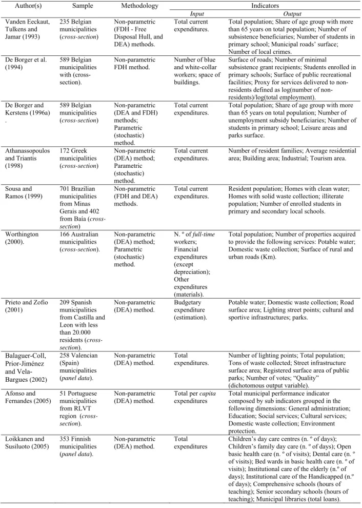
In Table 2 we survey studies that evaluate both non-parametrically and globally local governments’ efficiency. We can conclude that studies applying frontier analysis to the
7
For instance, for the Norwegian local government sector, Borge, Falch and Tovmo (2004) overcame this problem by using national cost weights to aggregate the main outputs of each municipality into a single aggregate output. These outputs were then divided by aggregate resources (measured in revenues) to get a measure of efficiency for each municipality.
9
local government sector do not abound in the literature, mainly because of the difficulty in defining local outputs and/or in obtaining statistical information to quantify all or at least several of them.8
As non-discretionary and discretionary inputs jointly contribute to outputs, there are in the literature several proposals on how to deal with this issue, implying usually the use of two-stage and even three-stage models.9 Some of the studies surveyed in Table 2 obtain efficiency scores from DEA using only controllable local inputs and outputs in the first stage and regress the efficiency scores on the non-discretionary inputs in a second stage as reported in Table 3.
The main purpose of these studies using regression models is to determine the impact of observable environmental variables on initial evaluation of local governments’ performance, providing a framework which allows non-discretionary inputs to feature in the explanation of differences in efficiency scores empirically estimated in the first stage. For instance, the results obtained by De Borger and Kerstens (1996a) and Balaguer-Coll, Prior-Jiménez and Vela-Bargues (2002) indicate that entities with higher tax revenues and/or those receiving higher grants are the most inefficient in the management of their resources.
8 For a literature review, see Worthington and Dollery (2000) and De Borger and Kerstens (2000). 9 See Ruggiero (2004) and Simar and Wilson (2004) for an overview.
10
Table 2 - Studies that evaluate both non-parametrically and globally local governments’ efficiency
Indicators
Author(s) Sample Methodology
Input Output Vanden Eeckaut, Tulkens and Jamar (1993) 235 Belgian municipalities (cross-section) Non-parametric (FDH - Free Disposal Hull, and DEA) methods.
Total current expenditures.
Total population; Share of age group with more than 65 years on total population; Number of subsistence beneficiaries; Number of students in primary school; Municipal roads’ surface; Number of local crimes.
De Borger et al. (1994) 589 Belgian municipalities with (cross-section). Non-parametric FDH method. Number of blue and white-collar workers; space of buildings.
Surface of roads; Number of minimal
subsistence grant recipients; Students enrolled in primary schools; Surface of public recreational facilities; Proxy for services delivered to residents defined as log(number of non-residents)/log(total employment). De Borger and Kerstens (1996a) . 589 Belgian municipalities (cross-section) Non-parametric (DEA and FDH) methods; Parametric (stochastic) method. Total current expenditures.
Total population; Share of age group with more than 65 years on total population; Number of unemployment subsidy beneficiaries; Number of students in primary school; Leisure areas and parks surface. Athanassopoulos and Triantis (1998) 172 Greek municipalities (cross-section) Non-parametric (DEA) method; Parametric (stochastic) method. Total current
expenditures. Number of resident families; Average residential area; Building area; Industrial; Tourism area.
Sousa and Ramos (1999) 701 Brazilian municipalities from Minas Gerais and 402 from Baía (cross-section) Non-parametric (FDH and DEA) methods. Total current expenditures.
Resident population; Homes with clean water; Homes with solid waste collection; illiterate population; Number of enrolled students in primary and secondary local schools. Worthington (2000). 166 Australian municipalities (cross-section). Non-parametric (DEA) method; Parametric (stochastic) method. N. º of full-time workers; Financial expenditures (except depreciation); Other expenditures (materials).
Total population; Number of properties acquired to provide the following services: Potable water; Domestic waste collection; Surface of rural and urban roads (Km).
Prieto and Zofio (2001)
209 Spanish municipalities from Castilla and Leon with less than 20.000 residents (cross-section). Non-parametric (DEA) method. Budgetary expenditure (estimation).
Potable water; Domestic waste collection; Road surface area; Lighting street points; cultural and sportive infrastructures; parks.
Balaguer-Coll, Prior-Jiménez and Vela-Bargues (2002) 258 Valencian (Spain) municipalities (panel data). Non-parametric
(DEA) method. Total expenditures. Number of lighting points; Total population; Tons of waste collected; Street infrastructure surface area; Registered surface area of public parks; Number of votes; “Quality”
(dichotomous output variable). Afonso and
Fernandes (2005) 51 Portuguese municipalities from RLVT region (cross-section).
Non-parametric
(DEA) method. Total per capita expenditures Total municipal performance indicator composed by sub indicators grouped in the following dimensions: General administration; Education; Social services; Cultural services; Domestic waste collection; Environment protection. Loikkanen and Susiluoto (2005) 353 Finnish municipalities (panel data). Non-parametric (DEA) method. Total expenditures
Children’s day care centres (n. º of days); Children’s family day care (n. º of days); Open basic health care (n. º of visits); Dental care (n. º of visits); Bed wards in basic health care (n. º of visits); Institutional care of the elderly (n.º of days); Institutional care of the Handicapped (n.º of days); Comprehensive schools (hours of teaching); Senior secondary schools (hours of teaching); Municipal libraries (total loans).
11
Table 3 – Studies that explain DEA efficiency scores with non-discretionary inputs
Regression results
Author(s) Country Positive impact on efficiency Negative impact on efficiency Vanden Eeckaut,
Tulkens and Jamar
(1993) Belgium
• High local tax rates; • Educational level of the adult
population.
• Higher per capita incomes and wealth of citizens;
• Per capita block grant;
• Political characteristics (number of coalition parties).
De Borger and Kerstens
(1996a) Belgium • • Local tax rates; Level of education.
• Per capita block grant; • Income.
Balaguer-Coll, Prior-Jiménez and Vela-Bargues (2002)
Spain • • Largest populations; Level of commercial activity.
• Higher per capita tax revenue; • Higher per capita grants. Athanassopoulos and
Triantis (1998) Greece • High share of fees and charges in municipal income; • High investment share in
total expenditures;
• Population density; • Grants;
• Parties affiliated to the central government.
Loikkanen and
Susiluoto (2005) Finland • Big share of municipal workers in age group 35-49 years;
• Dense urban structure; • High education level of
inhabitants.
• Peripheral location;
• High income level (high wages); • Large population;
• High unemployment; • Diverse service structure; • Big share of services bought from
other municipalities;
• A high share of costs covered by state grants reduced efficiency in first years after the end of matching grant era in 1993.
The efficiency scores estimated by De Borger and Kerstens (1996a) under several reference technologies were also explained by regression methods and the results were surprisingly similar. The level of taxation and education level also seem to be positively related to technical efficiency. By contrast, average income level and the ratio of grants to revenue were found to be negatively related to efficiency.
Additionally, Athanassopoulos and Triantis (1998) concluded that the most efficient municipalities were those that have high tax bases, income levels and public investment share on total expenditures. It was also found that inefficiency was related to high shares of grants in total municipal expenditures and population density.
12
Finally, Loikkanen and Susiluoto (2005) mention that factors such as peripheral location,10 large population, high levels of income and unemployment, and a big share
of services bought from other municipalities are negatively related to spending municipal efficiency. By contrast, high share of municipal workers in the age group of 35 to 49 years, narrow range of services, dense urban structure and high education level of population (proxy for education level of municipal workers in the basic service sectors) are factors that related positively to efficiency. A high share of state grants reduced efficiency, but after the 1997 reform leading to non-earmarked lump-sum grants, the grant variable was unrelated to efficiency.
3. DEA framework
We use the non-parametric method DEA, which was originally developed and applied to firms that convert inputs into outputs. Coelli, Rao and Battese (1998) and Sengupta (2000) introduce the reader to this literature and describe several applications.11 The term “firm”, sometimes replaced by the more encompassing Decision Making Unit (henceforth DMUs), the term coined by Charnes et al. (1978), may include non-profit or public organisations, such as hospitals, universities or local authorities.
Data Envelopment Analysis, originating from Farrell’s (1957) seminal work and popularised by Charnes, Cooper and Rhodes (1978), assumes the existence of a convex production frontier. The production frontier in the DEA approach is constructed using linear programming methods. The terminology “envelopment” stems out from the fact that the production frontier envelops the set of observations.12
10 This indicator was measured by the weighted average of road distances between the economic region of the municipality to all other domestic regions. In this measure pair-wise distances between regions are weighted with the Gross Regional Product of the destination region (cfr. Loikkanen and Susiluoto (2005). 11 A possible alternative non-parametric method would be Free Disposable Hull analysis (FDH). Deprins, Simar, and Tulkens (1984) first proposed the FDH analysis, which relaxes the convexity assumption maintained by the DEA model.
12 Technical efficiency is one of the two components of total economic efficiency, also referred to as X-efficiency. The second component is allocative efficiency and they are put together in the overall efficiency relation: economic efficiency = technical efficiency × allocative efficiency. A DMU is
technically efficient if it is able to obtain maximum output from a set of given inputs (output-oriented) or is capable to minimise inputs to produce the same level of output (input-oriented). On the other hand, allocative efficiency reflects the DMUs ability to use the inputs in optimal proportions. Coelli et al. (1998) and Thanassoulis (2001) offer introductions to DEA, while Simar and Wilson (2003) and Murillo-Zamorano (2004) are good references for an overview of frontier techniques.
13
The general relationship that we expect to test regarding efficiency can be given by the following function for each municipality i:
) ( i
i f X
Y = , i=1,…,n (1)
where we have Yi – indicators reflecting output measures; Xi – spending or other
relevant inputs in municipality i, either per inhabitant or in some other measure. IfYi < f(xi), it is said that municipality i exhibits inefficiency. For the observed input
level, the actual output is smaller than the best attainable one and inefficiency can then be measured by computing the distance to the theoretical efficiency frontier.
The purpose of an input-oriented example is to study by how much input quantities can be proportionally reduced without changing the output quantities produced. Alternatively, and by computing output-oriented measures, one could also try to assess how much output quantities can be proportionally increased without changing the input quantities used. The two measures provide the same results under constant returns to scale but give different values under variable returns to scale. Nevertheless, and since the computation uses linear programming, not subject to statistical problems such as simultaneous equation bias and specification errors, both output and input-oriented models will identify the same set of efficient/inefficient producers or DMUs.13
The analytical description of the linear programming problem to be solved, in the variable-returns to scale hypothesis, is sketched below for an input-oriented specification. Suppose there are k inputs and m outputs for n DMUs. For the i-th DMU, yi is the column vector of the inputs and xi is the column vector of the outputs. We can
also define X as the (k×n) input matrix and Y as the (m×n) output matrix. The DEA model is then specified with the following mathematical programming problem, for a given i-th DMU: 14
13 In fact, and as mentioned namely by Coelli, Rao and Battese (1998), the choice between input and output orientations is not crucial since only the two measures associated with the inefficient units may be different between the two methodologies.
14
We simply present here the equivalent envelopment form, derived by Charnes Charnes, Cooper and Rhodes (1978), using the duality property of the multiplier form of the original programming model.
14 0 1 ' 1 0 0 to s. min , ≥ = ≥ − ≥ + − λ λ λ θ λ θ λ θ n X x Y y i i . (2)
In problem (2), θ is a scalar (that satisfies θ≤ 1), more specifically it is the efficiency score that measures technical efficiency. It measures the distance between a municipality and the efficiency frontier, defined as a linear combination of the best practice observations. With θ<1, the municipality is inside the frontier (i.e. it is
inefficient), while θ=1 implies that the municipality is on the frontier (i.e. it is efficient).
The vector λ is a (n×1) vector of constants that measures the weights used to compute the location of an inefficient DMU if it were to become efficient. The inefficient DMU would be projected on the production frontier as a linear combination of those weights, related to the peers of the inefficient DMU. The peers are other DMUs that are more efficient and therefore are used as references for the inefficient DMU. n1 is a
n-dimensional vector of ones. The restriction n1'λ=1 imposes convexity of the frontier, accounting for variable returns to scale. Dropping this restriction would amount to admit that returns to scale were constant. Notice that problem (1) has to be solved for each of the n DMUs in order to obtain the n efficiency scores.
4. Relative municipal efficiency analysis
4.1. Data
In our analysis we assess the relative efficiency of individual Portuguese municipalities for 2001, within each of the aforementioned five “regions” defined according to the Portuguese nomenclature of territorial units with desegregation level II (NUTS II): Norte, Centro, Lisboa e Vale do Tejo (LVT), Alentejo and Algarve. The municipalities located in the Madeira and Azores islands were not included because their specific geographical location could raise comparability problems.
15
To use the DEA methodology, in order to derive efficiency measures, we need data on municipal inputs and outputs. As for the former, no measures on local production factors (such as labour or capital) used by local governments were available. To overcome this problem, we selected per capita municipal expenditures registered on municipal accounts for the year 2001 as a measure of the municipal resources used in local services’ provision. Input data for year 2001 were taken from the annual publication Municipal Finances: Application edited by the Portuguese Directorate-General of Local Governments.
Therefore, we are able to measure municipal spending efficiency (see Clements (2002)), not distinguishing technical from allocative efficiency. However, as the measurement of the latter requires price information, while the former only requires quantity data (Lovell (2000)), selecting per capita municipal spending gives us at least the guarantee that all inputs will be considered in our analysis (De Borger and Kerstens (2000)). Additionally, this variable is a more realistic municipal input measure if we acknowledge the reduced margin of manoeuvre that municipal authorities have to influence current expenditure choices, notably those concerning the compensation of employees.
As for municipal outputs, we use statistical information published in 2003 by the National Institute of Statistics (Instituto Nacional de Estatística) to construct a composite local government output indicator that tries to globally assess the several areas of municipal provision of services and goods. We explain in the next sub-section the construction of such output indicator.
4.2. Local Government Output Indicator (LGOI)
We focus on global municipal performance stemming from the municipal provision of several local services. However, as we were confronted with the difficulty of directly measuring some of the municipal production results, we concentrate on more homogenous basic local activities taking into account those spending functions enumerated in legal municipal government framework: rural and urban equipment, energy, transport and communications, education, patrimony, culture and science, sports
16
and leisure, healthcare, social services, housing, protection of the civil population, environment and basic sanitation, consumer protection, promote social and economic development, territory organisation, and external cooperation. Furthermore, some of the municipal performance indicators are surrogate measures of municipal services demand. The selection of indicators was based upon two general arguments implied within our analysis. First, municipalities with similar demand for homogeneous services should also have similar performance. Accordingly, we expect that a municipality with a younger population will allocate more public resources for the satisfaction of this particular group in terms, for example, of education and sportive services provision. Second, performance of municipal governments can be measured in terms of the improvement of observable factors directly controlled by municipal governments during the time period under consideration (see Lovell (1993)).
We present in Table 4 the selected output indicators (Yi) used to quantitatively proxy the results of individual municipal services provision (sources are provided in the Annex).
Table 4 – Selected municipal services indicators (Yi)
Variable Municipal Services Indicators
Y1 Social services - Local inhabitants with ≥ 65 years old, in percentage of the total resident population, 2001.
Y2 Education - School buildings per capita measured by the number of nursery and primary school buildings in percent of the total number of corresponding school-age inhabitants (Y21), 2001; - Gross primary enrolment ratio, the number of enrolled students in nursery and primary education in percent of the total number of corresponding school age inhabitants (Y22), 2001.
Y3 Cultural services - Number of library users in percentage of the total resident population, 2001.
Y4 Sanitation - Water supply, 1000 m3 (Y41); - Solid waste collection, tons (Y42).
Y5 Territory organisation - The number of licences for building construction, 2001. Y6 Road infrastructures - The length of roads maintained by the municipalities per
number of the total resident population, 1998.
Table 5 reports the regional average values for the selected municipal services indicators, suggesting the existence of large differences in performance across
17
Portuguese municipalities, mainly for cultural, sanitation and territory organisation services provision.
On average, municipalities located in the LVT region score well in sanitation and territory organisation service provision. By contrast, they have the lowest performance in basic education. As for infrastructure, municipalities of both LVT and Norte regions have the lowest scores. Therefore, since these regions siege the two main Portuguese cities – Lisbon (the capital) and Porto –, the measure of road infrastructure doesn’t apply in both cases because the administrative division of those cities matches the respective municipalities boundaries, which only include a single urban territory. From Table 5 it is possible to see that those municipalities belonging to Alentejo and Algarve regions seem to have a good performance in social and cultural services provision.
Table 5 – Regional average values for municipal result indicators (2001)
Basic Education
(Y2) Sanitation (Y4)
Region services Social (Y1) School buildings per capita (Y21) Education enrolment (Y22) Cultural services
(Y3) suWater pply (Y41) Waste collection (Y42) Territory organisation (Y5) Road infrastructures (Y6) Alentejo 0.257 0.023 0.626 1.149 1005.26 5639.66 83.26 0.020 Algarve 0.217 0.012 0.570 1.203 4280.19 18428.31 251.19 0.027 Centro 0.233 0.030 0.624 0.944 1864.24 8137.29 175.28 0.023 LVT 0.180 0.014 0.535 1.157 7811.96 36114.49 270.00 0.011 Norte 0.182 0.029 0.621 0.896 2708.06 18125.03 235.51 0.018 Min 0.180 0.012 0.535 0.896 1005.26 5639.66 83.26 0.011 Max 0.257 0.030 0.626 1.203 7811.96 36114.49 270.00 0.027
As suggested by several authors, we quantify the so-called Local Government Output Indicator (LGOI) as a single measure of municipal performance having in mind two objectives: on the one hand, to evaluate globally municipal performance; on the other hand, to carry with a frontier approach to local efficiency using that composite indicator as our output measure.15
The procedure adopted to construct the composite indicator for each region was as follows: first, all values of each sub-indicator mentioned in Table 4 were normalised by setting the average equal to one. Then, we compiled the performance indicator from the
18
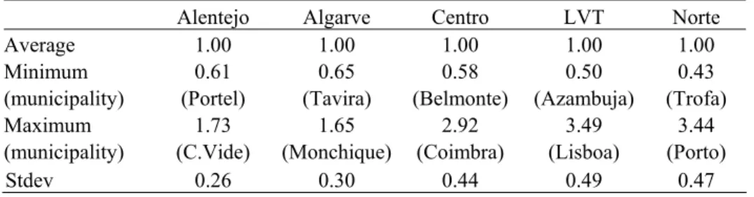
various sub-indicators giving equal weight to each of them. The summary values of our output measure, LGOI, observed within each of the five regions are reported in Table 6. These values refer to simple averages observed in the individual municipal results in each of the five regions considered in this study. The detailed set of results for our LGOI construction is presented in Appendix 1.
Table 6 – Regional summary values for LGOI - 2001
Alentejo Algarve Centro LVT Norte
Average 1.00 1.00 1.00 1.00 1.00
Minimum 0.61 0.65 0.58 0.50 0.43 (municipality) (Portel) (Tavira) (Belmonte) (Azambuja) (Trofa) Maximum 1.73 1.65 2.92 3.49 3.44 (municipality) (C.Vide) (Monchique) (Coimbra) (Lisboa) (Porto)
Stdev 0.26 0.30 0.44 0.49 0.47
Table 6 suggests large differences in municipal services provision performance within and across regions. Particularly, LVT, Centro and Norte regions show the highest standard deviation. These three regions are also those that on average spent less in 2001 in per capita terms (683.4, 812.04 and 682.34 euros respectively, as seen before in Table 1). By contrast, Algarve and Alentejo regions, although being less heterogeneous regions in terms of the LGOI, were the ones with the highest average spending per capita in 2001 (1128.78 and 982.71 euros respectively).
4.3. DEA results
In order to evaluate non-parametrically the efficiency in municipal provision on local services, we will use the LGOI as the output measure, and the level of per capita municipal spending as the input measure.
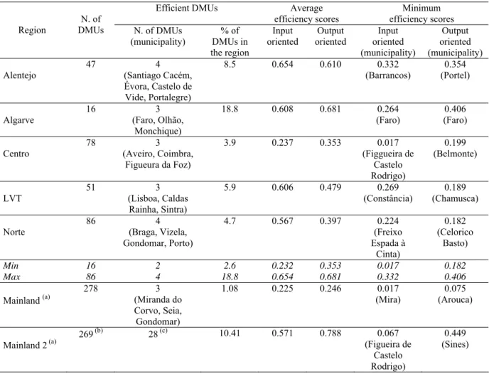
Table 7 summarizes our DEA results obtained with the one input, and one output, in all municipalities located within the five mainland regions, both in terms of input and output oriented efficiency scores for 2001. The individual and complete DEA results, for every municipality in each of the five regions, are presented in Appendix 2. We also report the DEA results regarding the entire set of municipalities in mainland Portugal, according to two alternative specifications: first, using, as for the five regions, a one
19
input and one output analysis; secondly, using instead of the aggregate LGOI measure its six sub-indicators as separate outputs.
Table 7 – DEA efficiency results
Efficient DMUs Average
efficiency scores
Minimum efficiency scores Region DMUs N. of N. of DMUs
(municipality) % of DMUs in the region Input oriented Output oriented Input oriented (municipality) Output oriented (municipality) Alentejo 47 (Santiago Cacém, 4
Évora, Castelo de Vide, Portalegre) 8.5 0.654 0.610 0.332 (Barrancos) (Portel) 0.354 Algarve 16 3 (Faro, Olhão, Monchique) 18.8 0.608 0.681 0.264 (Faro) 0.406 (Faro) Centro 78 (Aveiro, Coimbra, 3
Figueura da Foz) 3.9 0.237 0.353 0.017 (Figgueira de Castelo Rodrigo) 0.199 (Belmonte) LVT 51 3 (Lisboa, Caldas Rainha, Sintra) 5.9 0.606 0.479 0.269 (Constância) (Chamusca) 0.189
Norte 86 4 (Braga, Vizela,
Gondomar, Porto) 4.7 0.567 0.397 0.224 (Freixo Espada à Cinta) 0.182 (Celorico Basto) Min 16 2 2.6 0.232 0.353 0.017 0.182 Max 86 4 18.8 0.654 0.681 0.332 0.406 Mainland (a) 278 3 (Miranda do Corvo, Seia, Gondomar) 1.08 0.225 0.246 0.017 (Mira) (Arouca) 0.075 Mainland 2 (a) 269 (b) 28 (c) 10.41 0.571 0.788 0.067 (Figueira de Castelo Rodrigo) 0.449 (Sines)
Notes: The Mainland 2 DEA set of results was obtained using a one input and six outputs approach, where the several sub-indicators of the composite LGOI were used separately as outputs.
(a) The detailed DEA results for these two additional set of calculations, even if not presented here for space reasons, are available from the authors upon request.
(b) We excluded the municipalities for which data wasn’t available for at least one sub-indicator. Municipalities excluded for this reason were the following ones: Trofa, Porto, Ourique, Vizela, Marvão, Castro Marim, Murtosa, Odivelas and Lisboa.
(c) The twenty eight municipalities declared DEA efficient were the following ones: Alfândega da Fé, Aveiro, Boticas, Castro Daire, Coruche, Figueira da Foz, Idanha-a-Nova, Leiria, Mação, Mafra, Oliveira do Bairro, Paredes de Coura, Pedrógão Grande, Penalva do Castelo, Penamacor, Proença-a-Nova, Resende, Sabugal, São João da Madeira, Sardoal, Sintra, Torre de Moncorvo, Vila de Rei, Vila Nova de Cerveira, Vila Nova de Famalicão, Vila Real, Vila Velha de Ródão, Vinhais.
From Table 7 it is possible to see that the highest share of municipalities that would be labelled as most efficient and located on the theoretical production frontier within a given region belong to Algarve (Faro, Monchique and Olhão) and Alentejo (Santiago do
20
Cacém, Évora, Castelo de Vide and Portalegre). However, one has to bear in mind that these two regions are also the ones with the lower number of municipalities.
In what concerns the Norte region, which has the highest number of municipalities, only four municipalities (Braga, Vizela, Gondomar and Porto) were labelled as most efficient and located on the theoretical production frontier.
Interestingly for LVT region, the efficiency results confirm those obtained in Afonso and Fernandes (2005) in what concerns both the identification of the efficient municipalities (Lisbon, Caldas da Rainha and Sintra) and the input average efficiency score (around 0.6).
By comparing the averages of input efficiency scores observed within each of the five regions, we conclude that Alentejo (0.654) and Algarve (0.608) have the highest values, suggesting that their municipalities could theoretically achieve on average roughly the same level of local output with about 35.5 and 39.2 per cent fewer resources, respectively.
By contrast, municipalities belonging to Centro are reported in Table 7 as being the least efficient (0.232), implying that these municipalities could theoretically achieve on average roughly the same level of local output with about 76.8 per cent fewer resources, i.e., that local performance could be strongly improved without necessarily increasing municipal spending. Interestingly, it was also in this region that we observed both the lowest (128,37 euros for Figueira da Foz) and the highest (7683,33 euros for Figueira de Castelo Rodrigo) values for the selected input measure.
Considering the entire set of municipalities in mainland Portugal, we can compare the DEA results obtained using, on one hand, for each of the five regions, a one input and one output analysis (which we called “Mainland”), with those obtained using, on the other hand, a one input and six outputs specification, where the several sub-indicators of the composite LGOI were used separately (which we called “Mainland 2”). We may conclude that, as expected, the higher the number of factors included in the analysis (input and output variables), the higher the number of DMUs that are DEA declared
21
efficient.16 Indeed, the number of efficient municipalities and the average efficiency scores are both higher in Mainland 2 compared to Mainland DEA set of results.
5. Explaining inefficiency
5.1. Non-discretionary factors
One has to assume that some municipalities are unable to achieve the “best-practice” due to a relative harsh environment. Therefore, there is an interest in explaining the distribution of the efficiency scores previously calculated in the first-stage of our empirical analysis in light of local socio-economic and demographic specificities, as maintained, for example, by Bradford, Malt and Oates (1969), Schwab and Oates (1991), essentially mainly to help guiding public policy and assist municipal decision-making process.
Indeed, the standard DEA model as the one described in (1) incorporates only discretionary inputs, those whose quantities can be changed at the DMU will, and does not take into account the presence of environmental variables or factors, also known as non-discretionary inputs. However, socio-economic differences may play a relevant role in determining heterogeneity across the municipalities and influence performance outcomes. These exogenous socio-economic factors can include, for instance, the level of education of the population in a given region, the municipality’s purchasing power or even its geographical distance to the main decision centres.
In this sub-section our purpose is to empirically examine how the DEA efficiency results may be associated to, and thereby explained by, hypothesized factors proposed in the literature on local government sector efficiency. These factors can be broadly
16 These results support Banker et al. (1989) and Nunamaker (1985) argument that the number of DEA efficient DMUs varies positively as long as the difference between the number of observations and the number of variables increases. Pedraja-Chaparro et al. (1999) also affirm that “(...) other things being equal, a larger number of DMUs reduces the problem of data sparsity and increases the probability that the sample will include relatively efficient DMUs with which a poorly performing DMU can be compared”. As for the number of factors, these authors refer that “(...) other things being equal, as the number of factors increases, so the problem of data sparsity increases”.
22
identified under two main categories: inter-municipal competition and socioeconomic and demographic characteristics.
Regarding inter-municipal competition, for instance Tiebout (1956) and Heikkila (1996) argue that municipal inefficiency may be associated with the lack off competition pressures one municipality feels from other competing municipalities. This can arise because those competing forces can be related with the degree of choice mobile citizens/consumers do have to move into communities that offer a bundle of services that best match their own preferences.17 In fact, Loikkanen and Susiluoto (2005) found that peripheral location was negatively related to municipal spending efficiency. Following this trend, to approach these competitive forces we calculated the geographical distance between the municipality and its capital of district. This variable is expected to exert a negative effect on efficiency.
Bureaucracy inefficiency models (see Niskanen (1975) and Migué and Bélanger (1974)) envisage monitoring as a pragmatic framework to avoid the hypothesized tendency of local governments to pursue self-interests and political agenda (see, for instance, Mueller (2003), Hayes and Wood (1995) and Hayes, Razzolini and Ross (1998)). It has become common practice on local sector analysis the introduction of socio-economic and demographic characteristics that might explain variations in the ability of local residents to properly monitor local governments. These “community composition” elements may explain inter-municipal differences in the production of local goods consumed by local residents.
Although it is difficult to distinguish effects on demand from those determinants of inefficiencies, we may argue that efficiency may be affected by factors reflecting monitoring costs such as socio-economic factors. Indeed, the scope of “the disciplining
17
In fact, Hayes, Razzolini, and Ross (1998) and Grossman, Mavros and Wassmer (1999) findings support that intra-metropolitan suburban competition does positively contribute for the improvement of efficiency and it may be expected that metropolitan suburbs within closer proximity of each other enhance higher mobility choices than non-metropolitan municipalities, resulting from this “voting by feet” mechanism (Tiebout (1956)) higher pressures on local governments to be more efficient in the provision of local services. Additionally, Grossman, Mavros and Wassmer (1999)) argue that the more metropolitan suburban municipalities are perceived by mobile consumers as “effective substitutes” for metropolitan central city, the more technically efficient the central city tends to be.
23
effect of competition” (cfr. Grossman, Mavros and Wassmer (1999)) may be limited if monitoring the local government performance is difficult and costly due to, respectively, reduced ability of citizen-voters or the existence of opportunity costs to properly monitor local authorities (De Borger and Kerstens (1996a)).
Hamilton (1983) and Hayes, Razzolini, and Ross (1998) argue that local efficiency may depend on the ability of citizens to pressure local representatives and more specifically, that monitoring municipal performance, and even costs, depends on the education level of local residents.18 In what concerns spending efficiency, the findings of Vanden Eeckaut, Tulkens and Jamar (1993), De Borger and Kerstens (1996a) and Loikkanen and Susiluoto (2005) support the argument that efficiency is positively related to average level of education of local inhabitants. Therefore, we use two alternative measures of educational achievement: first, the percentage of population with secondary education; secondly, the percentage of population with tertiary education. We expect these variables to exert a positive effect in efficiency.19
To determine the impact of higher per capita incomes and wealth of citizens on spending efficiency we used the municipal per capita purchasing power, a per capita index estimated by the Portuguese National Institute of Statistics. The aim is then to assess whether richer local residents impose somehow an increased pressure in demanding more efficient local services.
In what concerns demographic characteristics, Grossman, Mavros and Wassmer (1999) argue that monitoring costs are likely to vary positively with geographic ‘sparsity of
18
Milligan, Moretti and Oreopoulos (2004) analyse the beneficial outcomes deriving from educational attainment, exploring the potential positive externalities of education as “enhanced political behaviour”. They find that education is related to several measures of political interest and involvement in U.S and U.K. This effect was supposed to be exercised through the following channels: (i) the “quality” of participation of a given subset of citizens (as Hamilton (1983)); and (ii) enlarged participation among citizens (or, as is the same, as being negatively related with what Grossman, Mavros and Wassmer (1999) labelled as “rationale ignorance” and “rationale abstention”, respectively). According to Milligan, Moretti, Oreopoulos (2004), “The first channel is important if education equips citizens with the cognitive skills they need to be effective participants in a representative democracy. In this case, education increases citizen’s ability to select able leaders, understand the issues upon which they will vote, act as a check on the potential excess of the government, and recognize corruption in leaders”.
19 According to Afonso and St. Aubyn (2005) this seems to be also the case in terms of cross country efficiency analysis.
24
municipalities’, which may indicate the presence of scale diseconomies. On the other hand, scale economies could exist when providing local public services for an enlarged number of residents, which would then increase its efficiency. We model this exogenous dimension by using population density variables and population growth.
5.2. Tobit analysis
Using the DEA output efficiency scores computed in the previous section, we now evaluate the importance of environmental or non-discretionary inputs. We present the results from Tobit estimations by regressing the output efficiency scores, δι, on a set of
possible explanatory variables as as follows
i i i i i i β β Y β E β D β Pop ε δ = 0 + 1 + 2 + 3 + 4 + , (3)
where, Y is a measure of purchasing power at the municipality level, E is a measure of the educational level, D is a variable that captures the effect of the geographical distance between the municipality and its capital of district, and Pop is a population related indicator, for instance population density of population growth.
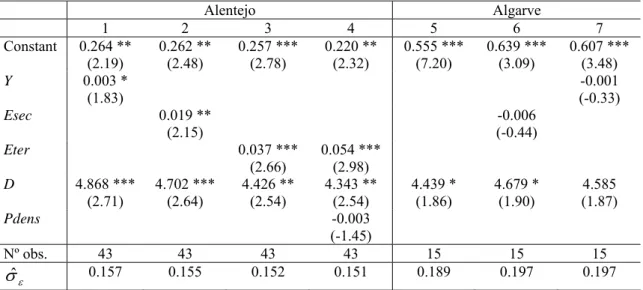
For a more simple reading of the results vis-à-vis the efficiency scores, we use the inverse of the geographical distance of each municipality to the capital of the respective district, which is then our variable D in (3). This means that a decrease in that distance increases its inverse and therefore would increase efficiency if the estimated coefficients for such variable were positive. We report in Tables 8, 9 and 10 the results from the censored normal Tobit regressions for several alternative specifications of equation (3) for each of the five regions plus overall estimations for the entire country (mainland). The results indicate that spending efficiency is positively and strongly related to the percentage of inhabitants with either secondary or tertiary education, across most regions and specifications, including the specification for the mainland (right-hand panel of Table 10). Furthermore, both variables had the same (positive) sign and were significant at 1 per cent level at least once, which indicates, firstly, that an increase in those variables would increase efficiency and, secondly, that the level of education has a
25
relevant impact on the efficiency of municipal provision. The only exception is the Algarve region, but one must bear in mind that this region has a much small number of DMUs, which limits the accuracy of the results.
Table 8 – Censored normal Tobit results: Alentejo and Algarve
Alentejo Algarve 1 2 3 4 5 6 7 Constant 0.264 ** (2.19) 0.262 ** (2.48) 0.257 *** (2.78) 0.220 ** (2.32) 0.555 *** (7.20) 0.639 *** (3.09) 0.607 *** (3.48) Y 0.003 * (1.83) (-0.33) -0.001 Esec 0.019 ** (2.15) (-0.44) -0.006 Eter 0.037 *** (2.66) 0.054 *** (2.98) D 4.868 *** (2.71) 4.702 *** (2.64) 4.426 ** (2.54) 4.343 ** (2.54) 4.439 * (1.86) 4.679 * (1.90) (1.87) 4.585 Pdens -0.003 (-1.45) Nº obs. 43 43 43 43 15 15 15 ε σˆ 0.157 0.155 0.152 0.151 0.189 0.197 0.197
Notes: Y – purchasing power; Esec – Population with secondary education; Eter – Population with tertiary education; D – distance to capital of district, inverse; PopDens – population density. The z statistics are in brackets. *, **, *** - Significant at the 10, 5 and 1 per cent level respectively. σˆε – Estimated standard deviation of ε.
Table 9 – Censored normal Tobit results: LVT, Norte
LVT Norte 1 2 3 4 5 6 7 Constant 0.341 *** (3.79) 0.374 *** (4.87) 0.421 *** (6.44) (1.60) 0.080 0.230 *** (4.91) 0.243 *** (5.47) 0.199 *** (3.84) Y 0.002 ** (2.44) 0.005 (6.45) *** Esec 0.010 ** (2.51) 0.016 (3.15) *** Eter 0.013 ** (2.97) 0.017 (2.27) ** 0.019 *** (2.68) D -1.897 ** (-2.10) -1.957 ** (-2.16) -1.979 ** (-2.16) (0.08) 0.023 8.77E-5 (2.60) *** PopDens 1.55E-4 ** (3.61) 7.21E-5 (2.17) ** PopVar 0.005 *** (2.81) 0.004 ** (2.33) Nº obs. 48 48 48 82 82 82 82 ε σˆ 0.106 0.177 0.178 0.160 0.168 0.151 0.149
Notes: Y – purchasing power; Esec – Population with secondary education; Eter – Population with tertiary education; D – distance to capital of district, inverse; PopDens – population density; PopVar – population variation. The z statistics are in brackets. *, **, *** - Significant at the 10, 5 and 1 per cent level respectively. σˆε – Estimated standard deviation of ε.
26
Table 10 – Censored normal Tobit results: Centro, Mainland
Centro Portugal (Mainland)
1 2 3 4 5 6 7 Constant 0.137 ** (2.05) 0.202 *** (3.36) 0.212 *** (2.91) 0.201 ** (2.18) 0.043 ** (2.09) 0.081 *** (3.52) 0.137 *** (4.78) Y 0.003 *** (3.38) 0.003 ** (2.24) 0.002 *** (2.61) 0.001 * (1.65) -2.03E-4 (-0.29) Esec 0.015 *** (3.23) 0.012 ** (2.09) Eter 0.013 *** (2.95) 0.011 *** (2.68) 0.014 *** (3.36) D -0.642 (-0.82) PopDens -1.042 (-1.30) 3.85E-5 *** (3.43) 5.27E-5 *** (4.47) PopVar 0.002 (0.60) (0.74) 0.002 0.002 (3.00) *** Nº obs. 78 78 78 78 278 278 278 ε σˆ 0.164 0.165 0.166 0.164 0.119 0.116 0.115
Notes: Y – purchasing power; Esec – Population with secondary education; Eter – Population with tertiary education; D – distance to capital of district, inverse; PopDens – population density; PopVar – population variation. The z statistics are in brackets. *, **, *** - Significant at the 10, 5 and 1 per cent level respectively. σˆε – Estimated standard deviation of ε.
For the purchasing power exogenous factor, used to assess whether richer local residents impose an increased pressure in demanding more efficient local services, the estimation results show positive and significant coefficients for all regions apart from Algarve.
It is also worthwhile mentioning that the estimates for population density revealed positive and significant coefficients for the Norte region and for the Mainland, indicating that a higher proportion of inhabitants living in dense settlement structures may facilitate the organization and consumption of networked local services. For all the other regions, this variable is not relevant in explaining inefficiencies. Population growth has a positive effect on efficiency also only for the Norte region and for the Mainland.
Finally, we found positive and statistically significant estimates for the coefficient of the geographical distance variable for the Alentejo, Algarve, and Norte regions. Hence, for those three regions, the closer the municipalities are to the capital of district the higher are their efficiency scores. On the other hand, this variable is not relevant either for the
27
Centro region of for the mainland. Interestingly, geographical distance impinges negatively on efficiency in the case of the LVT region, the more densely populated region (see Table 1), which includes the country’s capital. In other words, for this region, closeness to the capital may be undesirable for efficiency.
6. Conclusion
In this paper we evaluated public expenditure efficiency of Portuguese municipal governments in 2002, using Data Envelopment Analysis to compute input and output efficiency scores for the 278 Portuguese municipalities located in the mainland. The analysis is performed by clustering municipalities into the five “regions” defined for statistical purposes according to the Portuguese nomenclature of territorial units with desegregation level II (NUTS II): Norte, Centro, Lisboa e Vale do Tejo (LVT), Alentejo and Algarve.
To implement our frontier analysis we computed a so-called Local Government Output Indicator (LGOI) as a single measure of municipal performance, and used this composite indicator as our output measure for the DEA computations. Such composite indicator, also computed on a country (mainland) basis, includes sub-indicators of municipal services provision in the following areas: social services; education; cultural services; sanitation; territory organisations; and road infrastructures.
The results of the DEA calculations show that average regional input efficiency scores range from 0.237 in the Centro region to 0.654 in the Alentejo region. On the other hand, average regional output efficiency scores are between 0.353 in the Centro region and 0.681 in the Algarve region. On a municipal level, the evidence is naturally quite unequal, which implies that there is significant room for improvement in terms of possible theoretical efficiency gains. Regarding the five regions, as well as for the mainland model, the number of municipalities that define the efficiency frontier is between three and four.
Allowing for the separate use in the analysis of the output sub-indicators for the mainland, we find an overall input efficiency score of 0.571, which means that on
28
average it would be possible to attain the same level of output with roughly 43 per cent less of resources. Since the corresponding average output efficiency score is 0.788, a possible conclusion is that with the resources used, municipalities are on average producing some 21 per cent less in terms of public services than one would theoretically expect. Therefore, efficiency could be improved without necessarily increasing municipal spending. Additionally, under such model, and as one should expect, the number of municipalities that define the production possibility increases to twenty eight.
In order to see what factors may impinge on the efficiency level of municipal services provision, we performed a Tobit analysis both for each region and also for the mainland. Regarding the possible explanatory variables of inefficiencies in the provision of local governments’ services, the most relevant non-discretionary factors, which contribute positively to increase efficiency, seem to be: the level of education, either secondary or tertiary; municipal per capita purchasing power; and geographical distance.
Finally, one has to mention that these results should be put into some perspective, essentially because of two reasons. Firstly, the fact that some municipalities are not located on the theoretical production possibility frontier, and therefore not being labelled efficient, does not mean that they could actually be on the frontier. Indeed, municipal policy decisions may simply favour a different set of output provision. Secondly, the environmental factors, as discussed before, are a possible strong constraint to movements towards the production possibility frontier.
29
Appendix 1 – Detailed values for the LGOI measure
Table A1.1 – Local Government Output Indicator (LGOI): Alentejo, Algarve, LVT
Alentejo Algarve LVT
Municipality LGOI Municipality LGOI Municipality LGOI Aljustrel 0.84 Albufeira 1.08 Alcobaça 0.80
Almodôvar 1.34 Alcoutim 0.67 Bombarral 0.78 Alvito 1.04 Aljezur 1.11 Caldas da Rainha 0.89 Barrancos 1.10 Castro Marim 1.14 Nazaré 1.00 Beja 1.43 Faro 1.49 Óbidos 0.81 Castro Verde 1.04 Lagoa 1.03 Peniche 0.73 Cuba 1.40 Lagos 1.07 Alenquer 0.76 Ferreira do Alentejo 1.07 Loulé 1.35 Amadora 0.75 Grândola 1.09 Monchique 1.65 Arruda dos Vinhos 1.12 Mértola 0.84 Olhão 0.68 Cadaval 0.96 Moura 0.98 Portimão 0.94 Cascais 0.99 Odemira 1.32 São Brás de Alportel 0.89 Lisboa 3.49 Ourique 1.02 Silves 0.80 Loures 0.80 Santiago do Cacém 1.18 Tavira 0.65 Lourinhã 0.65 Serpa 0.88 Vila do Bispo 0.76 Mafra 1.12 Sines 0.94 Vila Real de Santo António 0.70 Odivelas 0.74 Vidigueira 0.92 Oeiras 1.07 Alandroal 0.87 Sintra 1.52 Alcacér do Sal 1.25 Sobral de Monte Agraço 1.35 Arraiolos 0.63 Torres Vedras 1.07 Borba 0.88 Vila Franca de Xira 0.90 Estremoz 0.97 Abrantes 0.69 Évora 1.70 Alcanena 1.06 Montemor-o-Novo 1.21 Almeirim 0.67 Mora 0.77 Alpiarça 0.93 Mourão 0.75 Azambuja 0.50 Portel 0.61 Benavente 0.79 Redondo 0.66 Cartaxo 0.69 Reguengos de Monsaraz 0.78 Chamusca 0.64 Vendas Novas 0.77 Constância 1.92 Viana do Alentejo 0.91 Coruche 2.18 Vila Viçosa 0.71 Entroncamento 0.96 Alter do Chão 1.14 Ferreira do Zêzere 0.96 Arronches 0.92 Golegã 0.97 Avis 0.68 Ourém 0.92 Campo Maior 0.84 Rio Maior 0.83 Castelo de Vide 1.73 Salvaterra de Magos 0.66 Crato 1.32 Santarém 0.93 Elvas 0.93 Sardoal 2.07 Fronteira 0.79 Tomar 0.79 Gavião 0.86 Torres Novas 0.73 Marvão 1.35 Vila Nova da Barquinha 0.95 Monforte 0.96 Alcochete 0.61 Nisa 0.82 Almada 1.37 Ponte de Sôr 1.05 Barreiro 0.74 Portalegre 0.95 Moita 1.01 Sousel 0.79 Montijo 0.61 Palmela 1.14 Seixal 1.02 Sesimbra 0.76 Setúbal 0.91
Average 1.00 Average 1.00 Average 1.00 Min (Portel) 0.61 Min (Tavira) 0.65 Min (Azambuja) 0.50
Max (Castelo de Vide) 1.73 Max (Monchique) 1.65 Max (Lisboa) 3.49
30
Table A1.2 – Local Government Output Indicator (LGOI): Centro, Norte
Centro Norte Municipality LGOI Municipality LGOI Municipality LGOI Municipality LGOI
Águeda 0.87 Sabugal 0.82 Arouca 0.65 Vila do Conde 1.01 Albergaria-a-Velha 0.77 Seia 0.84 Castelo de Paiva 0.61 Vila Nova de Gaia 1.84 Anadia 0.69 Trancoso 0.82 Espinho 1.06 Arcos de Valdevez 0.70 Aveiro 2.92 Alvaiázere 0.73 Oliveira de Azeméis 1.01 Caminha 1.00 Estarreja 0.73 Ansião 0.91 Santa Maria da Feira 0.97 Melgaço 1.19 Ílhavo 0.85 Batalha 0.89 São João da Madeira 1.53 Monção 0.69 Mealhada 0.94 Castanheira de Pêra 0.88 Vale de Cambra 0.72 Paredes de Coura 1.55 Murtosa 0.84 Figueiró dos Vinhos 0.89 Amares 0.60 Ponte da Barca 0.69 Oliveira do Bairro 1.35 Leiria 2.15 Barcelos 1.20 Ponte de Lima 1.17 Ovar 1.57 Marinha Grande 1.08 Braga 1.89 Valença 1.45 Sever do Vouga 0.83 Pedrógão Grande 1.14 Cabeceiras de Basto 0.59 Viana do Castelo 1.28 Vagos 0.88 Pombal 1.31 Celorico de Basto 0.55 Vila Nova de Cerveira 1.68 Belmonte 0.58 Porto de Mós 0.91 Esposende 1.01 Alijó 0.74 Castelo Branco 1.20 Mação 1.27 Fafe 0.88 Boticas 0.99 Covilhã 0.85 Carregal do Sal 0.79 Guimarães 1.61 Chaves 1.07 Fundão 1.11 Castro Daire 0.78 Póvoa de Lanhoso 0.58 Mesão Frio 1.19 Idanha-a-Nova 0.92 Mangualde 1.39 Terras de Bouro 0.64 Mondim de Basto 0.93 Oleiros 0.67 Mortágua 0.90 Vieira do Minho 0.65 Montalegre 0.98 Penamacor 0.72 Nelas 0.89
Vila Nova de
Famalicão 1.30 Murça 0.78 Proença-a-Nova 2.23 Oliveira de Frades 0.78 Vila Verde 0.90 Peso da Régua 0.55 Sertã 0.71 Penalva do Castelo 1.08 Vizela 0.61 Ribeira de Pena 0.72 Vila de Rei 0.90 Santa Comba Dão 0.92 Alfândega da Fé 0.77 Sabrosa 0.90 Vila Velha de Ródão 0.87 São Pedro do Sul 0.89 Bragança 2.03
Santa Marta de
Penaguião 0.82 Arganil 1.13 Sátão 0.64 Carrazeda de Ansiães 0.80 Valpaços 0.73 Cantanhede 1.47 Tondela 1.07
Freixo de Espada à
Cinta 0.74 Vila Pouca de Aguiar 0.72 Coimbra 2.92 Vila Nova de Paiva 0.86 Macedo de Cavaleiros 0.83 Vila Real 2.60 Condeixa-a-Nova 0.60 Viseu 1.68 Miranda do Douro 0.79 Armamar 0.73 Figueira da Foz 1.42 Vouzela 0.92 Mirandela 0.71 Cinfães 0.62 Góis 0.99 Mogadouro 0.65 Lamego 0.67 Lousã 0.84 Torre de Moncorvo 1.45 Moimenta da Beira 0.66 Mira 0.76 Vila Flor 1.13 Penedono 1.32 Miranda do Corvo 0.59 Vimioso 0.74 Resende 1.14 Montemor-o-Velho 0.78 Vinhais 0.73
São João da
Pesqueira 0.81 Oliveira do Hospital 0.70 Vila Nova de Foz Côa 0.67 Sernancelhe 0.75 Pampilhosa da Serra 0.87 Amarante 0.81 Tabuaço 0.98 Penacova 0.72 Baião 0.57 Tarouca 1.38 Penela 0.81 Felgueiras 0.84
Soure 0.71 Gondomar 1.27 Tábua 0.80 Lousada 0.65 Vila Nova de Poiares 1.27 Maia 1.02 Aguiar da Beira 0.90 Marco de Canaveses 0.95 Almeida 0.61 Matosinhos 1.63 Celorico da Beira 0.76 Paços de Ferreira 1.00 Fig. Castelo Rodrigo 0.64 Paredes 0.86 Fornos de Algodres 0.91 Penafiel 0.75 Gouveia 0.74 Porto 3.44 Guarda 1.12 Póvoa de Varzim 1.24 Manteigas 1.23 Santo Tirso 1.22 Meda 0.75 Trofa 0.43 Pinhel 0.67 Valongo 0.82
Average 1.00 Average 1.00
Min (Belmonte) 0.58 Min (Trofa) 0.43 Max (Coimbra) 2.92 Max (Porto) 3.44