DOI: http://dx.doi.org/10.1590/1678-992X-2017-0196
Sci. Agric. v.76, n.2, p.157-164, March/April 2019 ISSN 1678-992X
ABSTRACT: Soil physical quality in lowlands from the Pampa biome under no-tillage (NT) plays an important role; therefore, this study aimed to establish a soil physical quality index (SPQi) from a minimum data set to detect the effects of different deployment times of NT in an Albaqualf. The comparison of areas with one (NT1), three (NT3), five (NT5) and seven (NT7) years of no-tillage was established using as reference a non-cultivated field plot (NC) for at least thirty years, nearby the sites under NT. Soil samples with undisturbed and disturbed structure were collected to determine the physical quality indicators and soil organic matter (SOM) fractions. The factor analysis (FA) was used to identify and select a minimum data set. The SPQi was elaborated by using the deviations of the measured indicators at different deployment times of NT in relation to NC. The SPQi showed sensibility to identify and explain soil physical quality changes with different deployment times of NT. In well-drained lands, higher deployment times of no-tillage promote the physical quality of lowlands.
Keywords: factor analysis, minimum data set, management systems, lowland soils
Developing a Soil Physical Quality Index (SPQi) for lowlands under different deployment
Diony Alves Reis1* , Claudia Liane Rodrigues de Lima1 , Adilson Luís Bamberg2
1Universidade Federal de Pelotas/FAEM – Depto. de Solos, Campus Universitário s/n – 96050-500 – Pelotas, RS – Brasil.
2Embrapa Clima Temperado, Rod. BR 392, km 78 – 96010-971 – Pelotas, RS – Brasil.
*Corresponding author <[email protected]> Edited by: Silvia del Carmen Imhoff
Received May 30, 2017 Accepted October 05, 2017
Introduction
In Brazil, the Pampa biome occurs in Rio Grande do Sul State (RS), where 5.4 million hectares are low-lands, and Albaqualf is the predominant class (Parfitt et al., 2014). Albaqualf has high agricultural and economic importance due to its physical characteristics. The pres-ence of a subsurface layer almost impermeable, with expansive clays and low macro/microporosity ratio, fa-vor irrigated rice and livestock. Thus, the agricultural growth of the region is strongly dependent on under-standing soil physical properties in this environment.
Rainfed crops have been recently introduced into these soils, mostly cultivated under conventional tillage (CT) (Reis et al., 2016). The soybean has been an alter-native for the traditional flooded rice-livestock sequence, but there is a concern with the sustainability of this pro-duction model, as no-tillage (NT) has proven more profit-able and environmentally favorprofit-able in rainfed agriculture (Crittenden et al., 2015; Fernández-Romero et al., 2016; Raiesi and Kabiri, 2016) than other management systems.
Impacts of management systems on soil physical quality (SPQ) have been studied by the S index (Dexter, 2004), but its inconsistency has also been highlighted (van Lier, 2014; Moncada et al., 2015). In this sense, soil quality indices (SQI) were developed based on the ap-propriate selection of soil quality indicators to compose a minimum data set (MDS) (Karlen and Stott, 1994; Kar-len et al., 2001; Lima et al., 2008; Maia, 2013; Chen et al., 2013; Yao et al., 2013; Zornoza et al., 2015; Zhang et al., 2016; Rojas et al., 2016).
In MDS, attributes can be chosen by statistical methods (Paz-Kagan et al., 2014; Raiesi and Kabiri, 2016; Obade and Lal, 2016), such as the factor analysis (FA), which reduces redundant information from the original data set and groups soil attributes highly interrelated in
a smaller group of representative and independent attri-butes (Zhang et al., 2016; Raiesi and Kabiri, 2016), help-ing to understand the effects of changhelp-ing from CT to the NT system on soil physical quality.
Thus, given the agricultural importance of low-lands from the Pampa biome, this study aimed to es-tablish an MDS to develop a soil physical quality index (SPQi) and evaluate its sensitivity to different deploy-ment times of NT in Albaqualf from southern Brazil.
Materials and Methods
The study was carried out at the Lowland Ex-perimental Station – Embrapa Temperate Agriculture, located in Capão do Leão, RS, Brazil (31°49’04.13” S, 52°27’53.77” W, 14 m above sea level). The climate is
Cfa, according to Köppen classification (Alvares et al.,
2013), a hot mesothermal climate, with average temper-ature of coldest month between 3 and 18 °C. Average monthly rainfall is not below 60 mm, always humid, and average temperature of the hottest month higher than 22 °C. The soil was classified as Albaqualf (NRCS, 2010)
with 460 g kg–1 of sand, 370 g kg–1 of silt and 170 g kg–1
of clay within 0.0 to 0.2 m top layer.
The surface soil layer of the experimental area was historically managed under conventional tillage (CT). For this study, four experimental plots were selected and ho-mogenized before NT deployment through chisel plowing and soil acidity correction by superficial incorporation of dolomitic limestone using disc harrows. Then, different cover crops (Table 1) were established posteriorly, using 2
kg N ha–1, 26.2 kg P ha–1 and 49.8 kg ha–1 of mineral
fer-tilizer to summer crops and 15 kg N ha–1, 26.2 kg P ha–1,
49.8 kg ha–1 (base fertilization) and 100 kg N ha–1 (cover
fertilization) to summer and winter grasses. Furthermore, spontaneous plants were not fertilized.
Soils and Plant Nutrition
|
Resear
ch Ar
ticle
The study consists of five treatments, four NT [one (NT1), three (NT3), five (NT5) and seven (NT7) years un-der no-till] and a control treatment consisting of a 30-yr non-cultivated (NC) field located near the no-till treat-ments.
Soil samples with disturbed and undisturbed structure were collected from the 0.00 to 0.03; 0.03 to 0.06; 0.06 to 0.10 and 0.10 to 0.20 m soil layers. The sampled layers were defined in terms of their suscep-tibility to physical and hydric changes that originated from tillage and root systems activity of cultivated crops over the time.
Soil samples with undisturbed structure were collected with steel cylinders of 0.05 m diameter and 0.03 m height, totaling 240 samples (three cylinders for each layer × four soil layers × four replicates × five treatments). The soil samples were used to determine total porosity (TP), macroporosity (Ma), microporos-ity (Mi) (0.006 MPa to distinguish Ma and Mi by the tension table method), soil penetration resistance (PR) (Rousseau et al., 2013; D’Hose et al., 2014), bulk den-sity (Bd) (Merrill et al., 2013) and soil compressive
pa-rameters, preconsolidation pressure (σp), bulk density
at preconsolidation pressure (Bdσp), compression index
(CI) (Krümmelbein et al., 2010), degree of compactness
(Kondo and Dias Junior, 1999), at σp (DCσp, %) and at
1.600 kPa (DC1.600) (Reichert et al., 2016).
Soil samples with disturbed structure were col-lected, totaling 80 samples (one soil sample × four soil layers × four replicates × five treatments), to
deter-mine size classes of water-stable aggregates Ci, where i
represents1, 2, 3, 4, 5 classes (C1 = 9.51 to 4.76 mm;
C2 = 4.75 a 2.00 mm; C3 = 1.99 a 1.00 mm; C4 = 0.99 a 0.50 mm; C5 = 0.49 a 0.25 mm and C6 < 0.25 mm), Macroaggregates (Macro), Microaggregates (Micro), mean weight diameter of aggregates (MWD) (Kemper and Rosenau, 1986; Palmeira et al., 1999; Yoder, 1936), the free light fraction (FLF), the occluded light fraction (OLF) and the heavy fraction (HF) of organic matter contained in soil aggregates by performing the densi-metric fractionation of soil organic matter (SOM) (Imaz et al., 2010).
The total organic carbon content (TOC) was deter-mined (dry combustion - Perkin Elmer elemental ana-lyzer) in the densimetric fractions, and the carbon pool index (CPI), the carbon lability index (CLI) and the car-bon management index (CMI) were quantified.
The dataset included 24 indicators: TP, Ma, Mi, PR,
Bd, σp, CI, Bdσp, DCσp, DC1600, C2, C3, C4, C5,
Macro-aggregates, MicroMacro-aggregates, MWD, FLF, OLF, HF, TOC, CPI, CLI and CMI. The soil attributes were subjected to the factor analysis (FA) to identify highly correlated indi-cators for subsequent establishment of a minimum data set by eliminating attributes considered as redundant.
The FA was carried out using covariance (raw data) and correlation (standardized data) matrix. Vari-ables with sampling adequacy (Kaiser Criterion) < 0.5 were eliminated from the FA. Using the correlation ma-trix, factors with eigenvalues > 1 were retained and subjected to varimax rotation to maximize correlation between factors and measured attributes and to consti-tute the minimum data set (Yao et al., 2013; Mueller et al., 2013; Mota et al., 2014). The FA, the Communality and the SPQi were performed by PROC FACTOR and PROC ANOVA in SAS (Statistical Analyses System Insti-tute, version 9.2).
The Measure of Sampling Adequacy (MSA) indi-cates the proportion of variance in the variables caused by underlying factors. Values close to 1.0 (the measures can range from 0 to 1) generally indicate that the FA may be useful with the data while values lower than 0.5 indicate that the FA is probably not be suitable (Beavers et al., 2013).
Equation 1 was used to calculate the MSA value:
MSA i jr
i jr i ja ij
ij ij
=
+
∑
∑
∑
∑
∑
∑
2
2 2 1
MSA represents the ratio of the squared correla-tion between variables to the squared partial correlacorrela-tion
between variables (Kaiser, 1974), where: rij is the
cor-relation coefficient observed between variables i and j;
aijis the partial correlation coefficient between the same
variables that is, simultaneously, an estimate of the
cor-relation between the factors. The αij is probably close to
zero because factors are orthogonal to each other. The deviations of the measured attribute values in the areas under different deployment times of NT in re-lation to the reference values measured in the non-culti-vated field (NC) were calculated according to equation 2:
z x x s
i=
− 2
Table 1 – Crop sequence cultivated in an Albaqualf under different deployment times of no-tillage (NT).
Deployment times of NT Growing season
2007/08 2008/09 2009/10 2010/11 2011/12 2012/13
NT1 ... ... ... ... Ma Wh + Ma
NT3 ... ... Mi Rg + Sp + Sb Wh + Sb Wh + Sb
NT5 Ma Rg + Sp + Sb Wh + Sg Rg + Sp + Sb Wh + Sb Rg + Sp + Sb
NT7 Ma Wh + Sf Wh + Ma Rg + Sp + Sg Rg + Sp + Sb Rg + Sp + Sb
159
Reis et al. Soil quality index for lowland soils
Sci. Agric. v.76, n.2, p.157-164, March/April 2019
PR (r > 0.60), suggesting that compaction reduces the carbon content between and within aggregates and fa-vors the soil degradation process. In contrast, the TOC presented positive correlation with Ma (r = 0.77).
Askari and Holden (2015) evaluated 22 indicators of soil physical quality for assessing the effects of man-agement practices on SQ in temperate maritime soils, while Yao et al. (2013) used the Factor analysis (FA) to group 22 variables. According to Armenise et al. (2013), the FA general rules is to receive high eigenvalues (> 1.00) and to select variables with high factor loadings. These components allow to obtain the best parameter representative and retain it for screening of MDS (Chen et al., 2013; Yao et al., 2013; Zornoza et al., 2015; Zhang et al., 2016; Rojas et al., 2016).
The MSA values are used to keep or exclude at-tributes from the FA and are given in Table 3. Only 15 from the 24 soil attributes used initially were kept after the Kaiser criterion (MSA > 0.5). Despite the MSA
val-ues below 0.5, the following variables DCσp, DC1.600,
CPI and CLI were kept because the mean MSA value obtained for the set of variables was higher than 0.5. The FA was performed using a group of attributes with mean MSA higher than 0.5 thus using the parameters:
TP, Ma, Bd, PR, FLF, OLF, TOC, σp, CI, Bdσp, DCσp,
DC1600, CPI, CLI and CMI similarly to Yao et al. (2013) and Beniston et al. (2016).
Eigenvalues from the correlation matrix indicate that the first four factors explained > 98 % of total data variation (Table 4) (Yao et al., 2013; Paz-Kagan et al., 2014; Beniston et al., 2016; Basak et al., 2016).
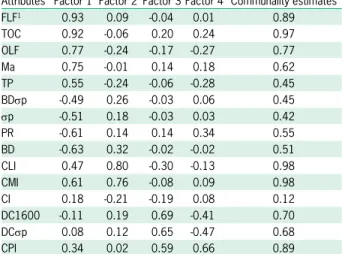
Factors with eigenvalue below 1 explain less vari-ance than an isolated soil attribute and therefore were refused according to the Kaiser Criterion (Armenise et al., 2013; Thomazini et al., 2015). The first factor, with eigen-value > 5, explained 53 % of total data variance (Table 4) with FLF and TOC, evidencing the higher positive load-ings (0.93 and 0.92, respectively). Nevertheless, contrast-ed with Bd and PR, that showcontrast-ed greater negative loadings (-0.63 and -0.61, respectively) (Table 5). Similarly, the sec-ond factor with an eigenvalue higher than one represents 17 % of total variability, where CLI and CMI evidenced higher positive loadings (0.80 and 0.76), contrasting with TP, OLF and CI, which showed greater negative loadings (-0.24, -0.24 and -0.21, respectively) (Table 5).
Considering the magnitude of the factorial load-ings of soil attributes presented in each factor, authors have named factors according to the relationship be-tween soil attributes and factors (Karlen et al., 2013; Gong et al., 2015). For example, factor 1 could be named as “Organic factor” because it presents positive factor loadings > 0.9, and the highest factor loadings were ob-served with attributes FLF and TOC. However, the fac-tors were not named in this study.
Greater communality estimates were observed in CLI and CMI (0.98) (Table 5), evidencing that these at-tributes share variability (Yao et al., 2013; Mueller et al., 2013), as well as TOC (0.97) and FLF (0.89).
Fur-where: zi is the standardized value selected by the FA
with mean (µ) and standard deviation (σ) equals to zero
and one, respectively; x is the value of the soil attribute
evaluated in the sites with different deployment times
of NT; xand s is the mean and the standard deviation,
respectively, of the soil attribute evaluated in NC.
To estimate the values of quality index (QIi) of the
each evaluated soil attribute, we used equations 3, 4 and 5 for the conditions “more is better”, “less is better”
and “midpoint optimum”, respectively, with β =
exp(-1,7145zi) (Maia, 2013).
The curve for the condition “more is better” has positive derivative and is used in indicators that improve soil quality, for example, total porosity, total organic car-bon, etc.; “midpoint optimum” has positive derivative until a maximum value and is used in indicators that positively affect soil quality until certain values that, if passed, cause negative influence such as bulk density, penetration resistance, etc. The curve for the condition “less is better” has negative derivative and is used in indicators that negatively affect the soil quality index, such as compactness degree (Chen et al., 2013; Naka-jima et al., 2015; Zhang et al., 2016).
QI= +
1
1 β 3
QI= +
β β
1 4
QI= +
4
1 2
β β
( ) 5
The soil physical quality index (SPQi) in each
eval-uated site was calculated by equation 6:
SPQi QI n i n n
i
=
∑
= 6where: QIiis the quality index of the evaluated
charac-teristic and n is the number of evaluated characteristics.
Soil quality evaluated with QIi, for the conditions “more
is better”, “less is better” and “midpoint optimum” and
without changes compared to the reference site has QIi
equal to one. Thus, values farther from one mean higher changes in relation to NC and reflecting these changes
in SPQi (Maia, 2013; Chen et al., 2013; Nakajima et al.,
2015; Zhang et al., 2016).
Results and Discussion
The analysis of 24 soil quality indicators of
Al-baqualf resulted in significant correlation (p < 0.05) in
172 of 276 soil attribute pairs (Table 2). Highest positive
correlation coefficients (r ≥ 0.80) were obtained for TP
160
Soil quality inde
x f
or lo
wland soils
.76, n.2, p.157-164, Mar
ch/April 2019
Mi Bd PR Macro MWD FLF OLF HF TOC CI σp BDσp DCσp DC1600 Ma C2 C3 C4 C5 Micro CPI CLI CMI
TP1 0.80** -0.39** -0.51** 0.12ns 0.35** 0.49** 0.56** 0.18** 0.43** 0.21** -0.31** -0.29** 0.09ns -0.01ns 0.40** 0.14ns -0.20** -0.29** -0.26** -0.16** -0.04ns 0.10ns 0.14ns
Mi -0.16* -0.30** 0.03ns 0.12ns 0.13ns 0.34** -0.17* 0.01ns 0.10ns -0.16* -0.13ns 0.04ns 0.00ns -0.15* 0.04ns -0.04ns -0.09ns -0.12ns -0.08ns -0.29** -0.06ns -0.12ns
Bd 0.45** -0.20** -0.39** -0.53** -0.54** -0.46** -0.59** -0.24** 0.38** 0.46** -0.02ns 0.12ns -0.47** -0.21** 0.13ns 0.28** 0.28** 0.22** -0.26** -0.05ns -0.15**
PR -0.20** -0.38** -0.52** -0.67** -0.20** -0.46** -0.03ns 0.32** 0.26** -0.06ns 0.05ns -0.40** -0.20** 0.15* 0.29** 0.25** 0.21** 0.09ns -0.25** -0.25**
Macro 0.45** 0.19** 0.16* 0.12ns 0.19** 0.00ns -0.11ns 0.07ns -0.03ns -0.01ns 0.23** 0.63** 0.37** 0.28** 0.05ns -0.97** 0.06ns 0.01ns 0.03ns
MWD 0.52** 0.36** 0.26** 0.48** 0.04ns -0.20** -0.25** 0.19** 0.14** 0.44** 0.16* -0.50** -0.65** -0.65** -0.43** 0.16* 0.17* 0.22**
FLF 0.72** 0.44** 0.89** 0.18* -0.41** -0.41** 0.05ns -0.10ns 0.69** 0.19** -0.33** -0.45** -0.32** -0.19** 0.28** 0.51** 0.63**
OLF 0.34** 0.67** 0.19** -0.41** -0.41** 0.03ns -0.13ns 0.48** 0.18* -0.15* -0.31** -0.21** -0.17* -0.01ns 0.24** 0.28**
HF 0.80** 0.04ns -0.30** -0.25** 0.06ns 0.03ns 0.61** 0.04ns -0.20** -0.23** -0.06ns -0.11ns 0.83** -0.13ns 0.18*
TOC 0.14* -0.43** -0.41** 0.07ns -0.06ns 0.77** 0.15* -0.32** -0.42** -0.24** -0.18* 0.59** 0.27** 0.51**
CI -0.06ns -0.11ns -0.14* -0.22** 0.16** 0.07ns 0.01ns -0.04ns -0.10ns -0.01ns -0.03ns -0.04ns -0.02ns
σp 0.46** -0.11ns 0.14* -0.35** -0.16* 0.10ns 0.16* 0.12ns 0.10ns -0.19** -0.12ns -0.18*
Bdσp -0.13ns 0.13ns -0.34** -0.07ns 0.26** 0.37** 0.24** -0.08ns -0.11ns -0.05ns -0.10ns
DCσp 0.73** 0.05ns 0.00ns -0.20** -0.22** -0.16** 0.04ns 0.09ns 0.02ns 0.06ns
DC1600 -0.05ns -0.03ns -0.13ns -0.13ns -0.11ns 0.01ns 0.10ns -0.06ns -0.02ns
Ma 0.21** -0.26** -0.33** -0.23** -0.21** 0.45** 0.27** 0.47**
C2 0.35** 0.18* -0.04ns -0.62** -0.02ns 0.10ns 0.11ns
C3 0.84** 0.34** -0.38** -0.20** -0.20** -0.26**
C4 0.51** -0.29** -0.14** -0.23** -0.27**
C5 -0.06ns 0.00ns -0.10ns -0.10ns
Micro -0.04ns 0.00ns -0.02ns
CPI -0.10ns 0.25**
CLI 0.92**
1TP = Total porosity (m3 m–3); Mi = Microporosity (m3 m–3); Bd = Bulk density (Mg m–3); PR = Penetration resistance (MPa); Macro = Macroaggregates (g kg–1); MWD = Mean weight diameter (mm); FLF = Carbon in the free
light fraction (g kg–1); OLF = Carbon in the occluded light fraction (g kg–1); HF = carbon in the heavy fraction (g kg–1); TOC = Total organic carbon (g kg–1); CI = Compression index (dimensionless); σp = preconsolidation
pressure (kPa); BDσp = Bulk density at preconsolidation pressure (Mg m–3); DCσp = Degree of compactness at preconsolidation pressure (%); DC1600 = Degree of compactness at pressure of 1600 kPa (%); Ma:
Macroporosity (m3 m–3); C2 = Size class of aggregates (4.75-2.00 mm); C3 = Size class of aggregates (1.99-1.00 mm); C4 = Size class of aggregates (0.99-0.50 mm); C5 = Size class of aggregates (0.49-0.25 mm);
Micro = microaggregates (g kg–1); CPI = Carbon pool index (dimensionless); CLI = Carbon lability index (dimensionless); CMI = Carbon management index (dimensionless); ns = non-significant difference; *,**significant
161
Reis et al. Soil quality index for lowland soils
Sci. Agric. v.76, n.2, p.157-164, March/April 2019
thermore, high values of communality estimate suggest that a high part of variance was explained by the factor. Lower values of communality estimate means no cor-relation or low corcor-relation, as observed in CI. Thus, CI was the least important attribute due to the lowest com-munality estimate.
Table 3 – Kaiser-Meyer-Olkin Measure of Sampling Adequacy (MSA)
of attributes of an Albaqualf under different deployment times of no-tillage (NT) in 0.00 to 0.20 m soil layer.
Attributes MSA
TP1 0.88
Bd 0.91
PR 0.88
FLF 0.80
OLF 0.85
TOC 0.73
CI 0.69
σp 0.80
BDσp 0.85
DCσp 0.48
DC1600 0.49
Ma 0.90
CPI 0.33
CLI 0.48
CMI 0.57
Mean MSA value 0.71
TP = Total porosity (m3 m–3); Bd = Bulk density (Mg m–3); PR = Penetration resistance (MPa); FLF = Carbon content in the free light fraction (g kg–1); OLF = Carbon content in the occluded light fraction (g kg–1); TOC = Total organic carbon content (g kg–1); CI = Compression index (dimensionless); σp = preconsolidation pressure (kPa); Bdσp = Bulk density at preconsolidation pressure (Mg m–3); DCσp = Degree of compactness at preconsolidation pressure (%); DC1600 = Degree of compactness at pressure of 1600 kPa (%); Ma = Macroporosity (m3 m–3); CPI = Carbon pool index (dimensionless); CLI = Carbon lability index (dimensionless); CMI = Carbon management index (dimensionless).
Table 4 – Eigenvalue, difference, proportion and cumulative variance
explained by factor analysis using correlation matrix (standardized data) for 0.00 to 0.20 m soil layer of an Albaqualf under different deployment times of no-tillage (NT).
Factors Eigenvalue Difference Proportion Cumulative %
1 5.21 3.53 0.53 53
2 1.68 0.19 0.17 70
3 1.49 0.27 0.15 86
4 1.22 0.84 0.12 98
5 0.38 0.16 0.04 100
6 0.22 0.08 0.02 100
7 0.13 0.07 0.01 100
8 0.06 0.05 0.01 100
9 0.01 0.03 0.00 100
10 -0.02 0.01 0.00 100
11 -0.02 0.03 0.00 100
12 -0.06 0.06 -0.01 100
13 -0.12 0.05 -0.01 100
14 -0.16 0.06 -0.02 100
15 -0.17 0.06 -0.02 100
Table 5 – Proportion of variance using varimax rotation and
communality estimates for soil attributes in the 0.00 to 0.20 m soil layer of an Albaqualf under different deployment times of no-tillage.
Attributes Factor 1 Factor 2 Factor 3 Factor 4 Communality estimates FLF1 0.93 0.09 -0.04 0.01 0.89
TOC 0.92 -0.06 0.20 0.24 0.97
OLF 0.77 -0.24 -0.17 -0.27 0.77
Ma 0.75 -0.01 0.14 0.18 0.62
TP 0.55 -0.24 -0.06 -0.28 0.45
BDσp -0.49 0.26 -0.03 0.06 0.45
σp -0.51 0.18 -0.03 0.03 0.42
PR -0.61 0.14 0.14 0.34 0.55
BD -0.63 0.32 -0.02 -0.02 0.51
CLI 0.47 0.80 -0.30 -0.13 0.98
CMI 0.61 0.76 -0.08 0.09 0.98
CI 0.18 -0.21 -0.19 0.08 0.12
DC1600 -0.11 0.19 0.69 -0.41 0.70
DCσp 0.08 0.12 0.65 -0.47 0.68
CPI 0.34 0.02 0.59 0.66 0.89
1FLF = Carbon content in the free light fraction (g kg–1); TOC = Total organic carbon content (g kg–1); OLF = Carbon content in the occluded light fraction (g kg–1); Ma = Macroporosity (m3 m–3); TP = Total porosity (m3 m–3); Bdσp = Bulk density at preconsolidation pressure (Mg m–3); σp = preconsolidation pressure (kPa); PR = Penetration resistance (MPa); Bd = Bulk density (Mg m–3); CLI = Carbon lability index (dimensionless); CMI = Carbon management index (dimensionless); CI = Compression index (dimensionless); DC1600 = Degree of compactness at pressure of 1600 kPa (%); DCσp = Degree of compactness at preconsolidation pressure (%); CPI = Carbon pool index (dimensionless).
The rotation of factors was applied to minimize the number of attributes with high factorial loadings within the same factor. Rotation also shows the relation of dependence between each other, negative or positive. High factorial loadings were observed in OLF (0.81), FLF (0.68), TP (0.64), Bd (-0.51) and PR (-0.71) in Factor 1, despite the positive and negative loadings. Therefore, the dependence between them was evident, as seen in their correlation coefficients (Table 2), suggesting that choosing one is enough to represent Factor 1 and the variables that compose it.
CLI and CMI presented positive loadings > 0.9 in Factor 2 while CPI, TOC and Ma showed positive
load-ings > 0.5. In Factor 4, DC1.600 and DCσp presented
positive loadings > 0.8 (Table 6).
According to the three standardization models (“less is better”, “more is better” and “midpoint optimum”), one parameter was selected per factor to compose the quality index of Albaqualf under different NT deployment times: Factor 1 (PR) “less is better”, Factor 3 (Ma) “midpoint
op-timum” and Factor 4 (DCσp) “less is better”. Attributes
for Factor 2 were not chosen, because the higher factor loading (> 0.9) were observed in CLI and CMI, which are already quality indexes of the Albaqualf compared to NC.
In general, a tendency of quality improvement of Albaqualf was seen with higher deployment times in all evaluated soil layers. This can be observed by greater
Ma and lower PR and DCp values, linked to the higher
through several characteristics that influence plant growth and development and considering the three selected pa-rameters, was promoted by the long term of NT. This is evident because of the high correlation coefficient (0.86,
p < 0.0001) between SPQi and higher deployment times
of NT (Figure 1).
Table 6 – Varimax orthogonal rotation of the factors for soil
attributes in 0.00 to 0.20 m soil layer of an Albaqualf under different deployment times of no-tillage.
Atributes Factor 1 Factor 2 Factor 3 Factor 4
OLF1 0.81 0.14 0.05 -0.08
FLF 0.68 0.46 0.38 -0.07
TP 0.64 0.02 0.01 0.02
BD -0.51 0.02 -0.28 0.10
PR -0.70 -0.15 0.05 -0.01
CLI 0.13 0.98 -0.08 0.00
CMI 0.15 0.94 0.27 0.03
CPI -0.11 0.00 0.93 0.08
TOC 0.61 0.25 0.68 -0.04
Ma 0.48 0.25 0.53 -0.04
DC1600 -0.02 -0.05 0.05 0.82
DCσp 0.07 0.00 0.02 0.81
CI 0.21 -0.07 0.03 -0.25
BDσp -0.30 -0.01 -0.10 0.02
σp -0.28 -0.08 -0.14 0.02
1OLF = Carbon content in the occluded light fraction (g kg–1); FLF = Carbon content in the free light fraction (g kg–1); TP = Total porosity (m3 m–3); Bd = Bulk density (Mg m–3); PR = Penetration resistance (MPa); CLI = Carbon lability index (dimensionless); CMI = Carbon management index (dimensionless); CPI = Carbon pool index (dimensionless); TOC = Total organic carbon content (g kg–1); Ma = Macroporosity (m3 m–3); DC1600 = Degree of compactness at pressure of 1600 kPa (%); DCσp = Degree of compactness at preconsolidation pressure (%); CI = Compression index (dimensionless); Bdσp = Bulk density at preconsolidation pressure (Mg m–3); σp = preconsolidation pressure (kPa).
Table 7 – Mean values, standard deviation (SD) and variation
coefficient (VC, %) Macroporosity (Ma), Penetration resistance (PR) and compactness degree at preconsolidation pressure (DCσp) of an Albaqualf at a non-cultivated field stie and under different deployment times of no-tillage (NT).
Ma PR DCσp
m3 m–3 MPa %
Non-cultivated field in the 0.00 to 0.03 m
Mean 9.10 0.73 91.01
SD 2.84 0.15 3.34
VC 31.24 20.26 3.66
Deployment time of NT
NT1 1.44 1.12 90.45
NT3 2.95 0.90 90.50
NT5 4.13 0.84 92.32
NT7 6.42 0.80 89.98
SPQi
NT1 0.04 0.16 0.55
NT3 0.10 0.32 0.51
NT5 0.20 0.33 0.57
NT7 0.52 0.35 0.48
Non-cultivated field in the 0.03 to 0.06 m
Mean 8.40 0.85 90.74
SD 3.14 0.22 5.14
VC 37.42 26.26 5.66
Deployment time of NT
NT1 1.97 1.44 86.42
NT3 3.24 1.12 91.94
NT5 3.91 1.03 90.95
NT7 6.16 0.97 88.74
SPQi
NT1 0.11 0.08 0.55
NT3 0.22 0.19 0.74
NT5 0.31 0.27 0.78
NT7 0.73 0.32 0.55
Non-cultivated field in the 0.06 to 0.10 m
Mean 8.34 0.89 93.43
SD 3.50 0.13 5.21
VC 41.96 14.40 5.58
Deployment time of NT
NT1 1.68 1.78 88.38
NT3 1.94 1.35 88.60
NT5 2.23 1.30 91.48
NT7 7.37 1.15 91.22
SPQi
NT1 0.14 0.00 0.55
NT3 0.17 0.04 0.68
NT5 0.19 0.05 0.82
NT7 0.87 0.23 0.74
Non-cultivated field in the 0.10 to 0.20 m
Mean 5.49 1.03 90.14
SD 1.12 0.15 4.41
VC 20.48 14.82 4.89
Deployment time of NT
NT1 2.08 2.21 90.09
NT3 2.10 1.72 90.92
NT5 2.67 1.56 90.45
NT7 3.96 1.52 91.01
SPQi
NT1 0.12 0.00 0.61
NT3 0.03 0.06 0.78
NT5 0.10 0.06 0.68
NT7 0.51 0.07 0.71
*NT1 = one; NT3 = three; NT = five and NT7 = seven years of NT deployment, respectively.
Figure 1 – Soil physical quality index (SPQi) for different layers
163
Reis et al. Soil quality index for lowland soils
Sci. Agric. v.76, n.2, p.157-164, March/April 2019
Considering that a better SPQi is equal to 1, NT7 showed the highest SPQi value (0.61) in 0.06 to 0.10 soil layer. In adjacent layers, the SPQi also increased with higher deployment times of NT; however, it tended to de-crease in at 0.10 to 0.20 m depth. In this study, deviations of attributes were evaluated in relation to NC, which does not necessarily mean that NC has optimal conditions. Al-though NC was even not grazed, and remained unman-aged during the last 30 years, NC is representative to a naturally restored area, not a native field.
The SPQi has shown sensitivity and ability to de-tect changes resulting from soil tillage practices (Figure 1) (Mukherjee and Lal, 2014; Mota et al., 2014; Askari and Holden, 2015; Crittenden et al., 2015; Duval et al., 2016). The evaluated tool has shown that higher deploy-ment time of NT promoted the physical quality of the Albaqualf. Furthermore, the SPQi has shown efficiency to evaluate soil quality. Moreover, it can be used to com-pare areas subjected to different practices and cultivation conditions.
The physical improvement of lowlands evaluated in this study was demonstrated through several indicators, in particular through that SPQi, which compiled the informa-tion of many indicators. The SPQi has shown the ability of NT to ameliorate lowlands for a better adaptation of high-land crops in the Pampa biome, as well as to promote soil ecological and conservation functions (i.e. carbon fixation, water infiltration and aeration, drainage regulation and erosion prevention). These benefits are similar to those ob-served in Brazilian well-drained lands cultivated under NT.
Conclusion
The present study has demonstrated the efficiency of the factorial analysis in selecting the parameters to con-stitute a minimum data set to evaluate soil quality under different deployment times of no-till. The soil physical quality index (SPQi), constructed from macroporosity, soil resistance to penetration and the compaction degree in the preconsolidation pressure were sensitive to reflect soil physical quality improvements of Albaqualf. This study has also showed that the improvement of physical quality from a cropped Albaqualf is highly dependent of organic matter accumulation in soil surface layers. No-tillage also generated and preserved roots derived and interaggregate macropores, which are essential for gas diffusion and rapid flow of internal water drainage in these soils. Regardless of inherent differences between soil types, the benefits of no tillage for physical status of the studied Albaqualf were comparable to those in Brazilian Oxisols.
Acknowledgments
To Coordenação de Aperfeiçoamento de Pessoal de Nível Superior (CAPES) for a scholarship granted to the first author; to the Federal University of Pelotas and Em-brapa Temperate Agriculture for the opportunity, finan-cial and laboratory support and infrastructure.
Authors’ Contributions
Conceptualization: Bamberg, A.L. Data Acquisi-tion: Reis, D.A., Bamberg, A.L. Data Analysis: Reis, D.A. Design of Methodology: Lima, C.L.R. Writing and Edit-ing: Reis, D.A., Lima, C.L.R., Bamberg, A.L.
References
Alvares, C.A.; Stape, J.L.; Sentelhas, P.C.; Gonçalves, J.L.M.; Sparovek, G. 2013. Köppen’s climate classification map for Brazil. Meteorologische Zeitschrift 22: 711-728.
Armenise, E.; Redmile-Gordon, M.A.; Stellacci, A.M.; Ciccarese, A.; Rubino, A.P. 2013. Developing a soil quality index to compare soil fitness for agricultural use under different managements in the Mediterranean environment. Soil and Tillage Research 130: 91-98.
Askari, M.S.; Holden, N.M. 2015. Quantitative soil quality indexing of temperate arable management systems. Soil and Tillage Research 150: 57-67.
Basak, N.; Datta, A.; Mitran, T.; Roy, S.S.; Saha, B.; Biswas, S.; Mandal, B. 2016. Assessing soil-quality indices for subtropical rice-based cropping systems in India. Soil Research 54: 20-29.
Beavers, A.S.; Lounsbury, J.W.; Richards, J.K.; Huck, S.W.; Skolits, G.J.; Esquivel, S.L. 2013. Practical considerations for using exploratory factor analysis in educational research. Practical Assessment, Research and Evaluation 18: 1-13.
Beniston, J.W.; Lal, R.; Mercer, K.L. 2016. Assessing and managing soil quality for urban agriculture in a degraded vacant lot soil. Land Degradation & Development 27: 996-1006.
Chen, Y.; Wang, H.; Zhou, J.; Xing, L.; Zhu, B.; Zhao, Y.; Chen, X. 2013. Minimum data set for assessing soil quality in farmland
of northeast China. Pedosphere23: 564-576.
Crittenden, S.J.; Poot, N.; Heinen, M.; van Balen, D.J.M.; Pulleman, M.M. 2015. Soil physical quality in contrasting tillage systems in organic and conventional farming. Soil and Tillage Research 154: 136-144.
D’Hose, T.; Cougnon, M.; De Vliegher, A.; Vandecasteele, B.; Viaene, N.; Cornelis, W.; Van Bockstaele, E.; Reheul, D. 2014. The positive relationship between soil quality and crop production: a case study on the effect of farm compost application. Applied Soil Ecology 75: 189-198.
Dexter, A.R. 2004. Soil physical quality. I. Theory, effects of soil texture, density, and organic matter, and effects on root growth. Geoderma 120: 201-214.
Duval, M.E.; Galantini, J.A.; Martínez, J.M.; López, F.M.; Wall, L.G. 2016. Sensitivity of different soil quality indicators to assess sustainable land management: influence of site features and seasonality. Soil and Tillage Research 159: 9-22.
Fernández-Romero, M.L.; Clark, J.M.; Collins, C.D.; Parras-Alcántara, L.; Lozano-García, B. 2016. Evaluation of optical techniques for characterizing soil organic matter quality in agricultural soils. Soil and Tillage Research 155: 450-460.
Imaz, M.J.; Virto, I.; Bescansa, P.; Enrique, A.; Fernandez-Ugalde, O.; Karlen, D.L. 2010. Soil quality indicator response to tillage and residue management on semi-arid Mediterranean cropland. Soil and Tillage Research 107: 17-25.
Kaiser, H.F. 1974. An index of factorial simplicity. Psychometrika 39: 32-35.
Karlen, D.L.; Andrews, S.S.; Doran, J.W. 2001. Soil quality: current concepts and applications. Advances in Agronomy 74: 1-40. Karlen, D.L.; Kovar, J.L.; Cambardella, C.A.; Colvin, T.S. 2013.
Thirty-year tillage effects on crop yield and soil fertility indicators. Soil and Tillage Research 130: 24-41.
Karlen, D.L.; Stott, D.E. 1994. A framework for evaluating physical and chemical indicators of soil quality. p. 53-72. In: Doran, J.W.; Coleman, D.C.; Bezdicek, D.F.; Stewart, B.A., eds. Defining soil quality for a sustainable environment. Soil Science Society of America, Madison, WI, USA. (SSSA Special Publication, 35). Kemper, W.D.; Rosenau, R.C. 1986. Aggregate stability and size
distribution. p. 425-441. In: Klute, A., ed. Methods of soil analysis. 2ed. Soil Science Society of America, Madison, WI, USA.
Kondo, M.K.; Dias Junior, M.S. 1999. Management and moisture effects on the compressive behavior of three latosols (oxisols). Brazilian Journal of Soil Science 23: 497-506 (in Portuguese, with abstract in English).
Krümmelbein, J.; Horn, R.; Raab, T.; Bens, O.; Hüttl, R.F. 2010. Soil physical parameters of a recently established agricultural recultivation site after brown coal mining in eastern Germany. Soil and Tillage Research 111: 19-25.
Lima, A.C.R.; Hoogmoed, W.B.; Brussaard, L. 2008. Soil quality assessment in rice production systems: establishing a minimum data set. Journal of Environmental Quality 37: 623-630. Maia, C.E. 2013. Environmental quality in soil with different
growing season cultivated w ith muskmelon irrigated. Ciência Rural 43: 603-609 (in Portuguese, with abstract in English). Merrill, S.D.; Liebig, M.A.; Tanaka, D.L.; Krupinsky, J.M.; Hanson,
J.D. 2013. Comparison of soil quality and productivity at two sites differing in profile structure and topsoil properties. Agriculture, Ecosystems and Environment 179: 53-61.
Moncada, M.P.; Ball, B.C.; Gabriels, D.; Lobo, D. 2015. Evaluation of soil physical quality index S for some tropical and temperate medium-textured soils. Soil Science Society of America Journal 79: 9-19.
Mota, J.C.A.; Alves, C.V.O.; Freire, A.G.; Assis Júnior, R.N. 2014. Uni and multivariate analyses of soil physical quality indicators of a Cambisol from Apodi Plateau - CE, Brazil. Soil and Tillage Research 140: 66-73.
Mueller, L.; Shepherd, G.; Schindler, U.; Ball, B.C.; Munkholm L.J.; Hennings, V.; Smolentseva, E.; Rukhovic, O.; Lukin, S.; Hui, C. 2013. Evaluation of soil structure in the framework of an overall soil quality rating. Soil and Tillage Research 127: 74-84. Mukherjee, A.; Lal, R. 2014. Comparison of soil quality index using
three methods. PloS One 9: e105981.
Nakajima, T.; Lal, R.; Jiang, S. 2015. Soil quality index of a Crosby silt loam in central Ohio. Soil and Tillage Research 146: 323-328. Natural Resources Conservation Service [NRCS]. 2010. Keys to
Soil Taxonomy. 11ed. United States Department of Agriculture, Washington, DC, USA.
Obade, V.P.; Lal, R. 2016. A standardized soil quality index for diverse field conditions. Science of the Total Environment 541: 424-434.
Palmeira, P.R.T.; Pauletto, E.A.; Teixeira, C.F.A.; Gomes, A.S.; Silva, J.B. 1999. Soil aggregation of an Albaqualf submitted to different soil tillage systems. Revista Brasileira de Ciência do Solo 23: 189-195 (in Portuguese, with abstract in English).
Parfitt, J.M.B.; Timm, L.C.; Reichardt, K.; Pauletto, E.A. 2014. Impacts of land leveling on lowland soil physical properties. Revista Brasileira de Ciência do Solo 38: 315-326.
Paz-Kagan, T.; Shachak, M.; Zaady, E.; Karnieli, A. 2014. A spectral soil quality index (SSQI) for characterizing soil function in areas of changed land use. Geoderma 171-184.
Raiesi, F.; Kabiri, V. 2016. Identification of soil quality indicators for assessing the effect of different tillage practices through a soil quality index in a semi-arid environment. Ecological Indicators 71: 198-207.
Reichert, J.M.; Rosa, V.T.; Vogelmann, E.S.; Rosa, D.P.; Hornd, R.; Reinert, D.J.; Sattlere, A.; Denardin, J.E. 2016. Conceptual framework for capacity and intensity physical soil properties affected by short and long-term (14 years) continuous no-tillage and controlled traffic. Soil and Tillage Research 158: 123-136. Reis, D.A.; Lima, C.L.R.; Bamberg, A.L. 2016. Physical quality and
organic matter fractions of an Alfisol under no-tillage. Pesquisa Agropecuária Brasileira 51: 1623-1632 (in Portuguese, with abstract in English).
Rojas, J.M.; Prause, J.; Sanzano, G.A.; Arce, O.E.A.; Sánchez, M.C. 2016. Soil quality indicators selection by mixed models and multivariate techniques in deforested areas for agricultural use in NW of Chaco, Argentina. Soil and Tillage Research 155: 250-262.
Rousseau, L.; Fonte, S.J.; Téllez, O.; Van der Hoek, R.; Lavelle, P. 2013. Soil macrofauna as indicators of soil quality and land use impacts in smallholder agroecosystems of western Nicaragua. Ecological Indicators 27: 71-82.
Thomazini, A.; Mendonça, E.S.; Cardoso, I.M.; Garbin, M.L. 2015. SOC dynamics and soil quality index of agroforestry systems in the Atlantic rainforest of Brazil. Geoderma Regional 5: 15-24.
Van Lier, Q. de J. 2014. Revisiting the S-index for soil physical
quality and its use in Brazil. Revista Brasileira de Ciência do Solo 38: 1-10.
Yao, R.; Yang, J.; Gao, P.; Zhang, J.; Jin, W. 2013. Determining minimum data set for soil quality assessment of typical salt-affected farmland in the coastal reclamation area. Soil and Tillage Research 128: 137-148.
Yoder, R.E. 1936. A direct method of aggregate analysis of soil and a study of the physical nature of erosion losses. Journal of American Society of Agronomy 28: 337-351.
Zhang, G.; Bai, J.; Xi, M.; Zhao, Q.; Lu, Q.; Jia, J. 2016. Soil quality assessment of coastal wetlands in the Yellow River Delta of China based on the minimum data set. Ecological Indicators 66: 458-466.