Symplectic Integration Methods in Molecular
and Spin Dynamics Simulations
Shan-Ho Tsai
a,b, M. Krech
c, and D.P. Landau
a aCenter for Simulational Physics, University of Georgia, Athens, GA 30602, USA
b
Enterprise Information Technology Services, University of Georgia, Athens, GA 30602, USA
c
Max-Planck-Institut f¨ur Metallforschung, Stuttgart 70569, Germany
Received on 2 September, 2003
We review recently developed decomposition algorithms for molecular dynamics and spin dynamics simula-tions of many-body systems. These methods are time reversible, symplectic, and the error in the total energy thus generated is bounded. In general, these techniques are accurate for much larger time steps than more stan-dard integration methods. Illustrations of decomposition algorithms performance are shown for spin dynamics simulations of a Heisenberg ferromagnet.
1
Introduction
Molecular dynamics[1] and spin dynamics[2] simulations are powerful tools for investigating the time evolution of physical quantities and hence enhancing our understanding of dynamic properties of many-body systems. In these sim-ulations the classical equations of motion governing the dy-namical properties of the systems are solved numerically, with restrictions given by some initial conditions. Typically the time scale of the phenomena of interest is much longer than the time steps that can be used in standard finite time difference methods. Therefore, a large number of total inte-gration steps is required, and this generates large truncation errors unless the time step used is very small. Small time steps often lead to forbiddingly long integrations.
Progress was accelerated with the advent of new, sym-plectic methods for integrating coupled equations of mo-tion [3-6]. These numerical algorithms are based on de-compositions of exponential operators. They are time re-versible, symplectic (i.e they conserve exactly the invari-ant phase-space volume) and the error in the total energy of the system is bounded[7, 8]. (In some cases the total energy of the system is conserved exactly[9, 10].) The ef-fectiveness and efficiency of these symplectic methods have been illustrated with spin dynamics simulations of the mag-netic excitations in RbMnF3 using a fourth-order
Suzuki-Trotter decomposition method[6, 9]. The improved integra-tion method has been used to obtain high-resoluintegra-tion results, which could, for the first time, be compared directly and quantitatively with neutron-scattering data, yielding good agreement and shedding light onto controversies between theory and experiment[11].
In this paper we review decomposition algorithms ap-plied to classical molecular dynamics and spin dynamics simulations. In Section II we express the classical equa-tions of motion used in molecular dynamics in the Liouville formulation and in Section III we introduce spin dynamics
simulations. We discuss criteria for good integration meth-ods in Section IV and we briefly review a few standard inte-gration algorithms in Section V. In Section VI we describe the new decomposition algorithms and show some numer-ical tests and in Section VII we present spin dynamics re-sults for RbMnF3. Finally, a summary is provided in Section
VIII.
2
Molecular Dynamics
Let us consider a system ofNparticles with massesmi de-scribed by their positionsriand velocitiesvi, interacting via a potentialu(rij), whererij = ri−rj. The Hamiltonian function of the system can be written as
H= N
i=1
1 2miv
2
i +
i,j, j=i
u(rij), (1)
and the force on particleidue to particlejis given by
fij=−∇riu(rij) =−
∂u(rij)
∂rij
rij
rij.
(2) The equations of motion are given by
mi
d2r
i
dt2 =
j, j=i
fij ≡fi, i= 1, .., N. (3)
The time evolution of the system can be studied by integrat-ing the equations of motion to obtainri(t)andvi(t), for
i = 1,2,· · ·, N, and by expressing other physical quanti-ties in terms ofri(t)andvi(t).
2.1
Liouville Formulation
The equations of motion (3) can be rewritten as
dy
wherey(t) = {ri(t),vi(t)}denotes a configuration of the
N particles, andLˆis the Liouville operator defined as
ˆ L≡ N i=1
vi·
∂ ∂ri
+ fi
mi · ∂
∂vi
≡A+B (5)
The termN
i=1vi· ∂∂ri ≡ Ain Eq.(5) corresponds to the
free motion of the particles (kinetic part), whereas the po-tential part is given by the termN
i=1
fi
mi · ∂
∂vi ≡B. With
these definitions of operatorsAandB, the equations of mo-tion (4) can be written as
dy
dt = (A+B)y(t), (6)
which have the formal solution
y(t+ ∆) = e(A+B)∆y(t), (7) where∆represents a time step. For a general many-body system the combined operatione(A+B)∆y(t)cannot be
eas-ily performed. However, the separate operatorseA∆y and
eB∆ycan be written as
eA∆y= exp
∆ N
i=1
vi·
∂ ∂ri
{ri,vi}={ri+vi∆,vi} (8) eB∆y= exp
∆ N i=1 fi mi · ∂
∂vi
{ri,vi}={ri,vi+
fi
mi ∆}
(9) and they represent shifts in the positions and in the veloci-ties, respectively. Moreover, the shift in the positions (ve-locities) generated byeA∆y(eB∆y) only depends on the
ve-locities (positions) and can be easily computed. However, note that in generale(A+B)∆ = eA∆eB∆!
3
Spin Dynamics
For simplicity, let us discuss spin dynamics simulations for a specific spin model, namely the classical isotropic Heisen-berg model, described by the Hamiltonian
H=−J
i,j
Si·Sj (10)
where Si is a unit vector located on a lattice site i, and nearest-neighbor pairs of spins are coupled with an inter-action parameterJ, which can be ferromagnetic (J >0) or antiferromagnetic (J < 0). One of the best physical real-izations of this model is RbMnF3, where the magnetic ions
Mn+2have spinS = 5/2, and are located on the sites of a simple cubic lattice. Nearest-neighbor interactions are anti-ferromagnetic, withJexp=−(0.58±0.06)meV. Magnetic
ordering with antiferromagnetic alignment of spins occurs below the critical temperatureTc = 83K. For the discus-sions in this section we will consider simple cubic lattices with periodic boundary conditions.
Unlike the Ising model (Si = ±1), Heisenberg models have true dynamics governed by the equations of motion
dSi
dt =−Si× ∂H
∂Si
(11) which can be rewritten as
dSi
dt =−Si×Heffi (12)
where the effective fieldHeffiis defined as
Heffk i=−J
j=N N(i)
Sjk, k=x, y, z (13)
with the sum performed over all nearest-neighbor sites ofi. If we denote
Si= Sx i
Siy
Sz i (14)
we can then write the equations of motion as
dSi
dt =
0 −Hz
effi H y
effi
Hz
effi 0 −H x
effi
−Heffy i Hx
effi 0
Si≡RSi (15)
for which the formal solution is
Si(t+ ∆) = eR∆Si(t), (16) where∆represents a time step.
Spin dynamics simulations can be used to study several dynamic properties of classical spin systems[2]. Of partic-ular interest are the dynamic structure factors, which are Fourier transforms of space- and time-displaced spin-spin correlation functions given by
Ck(r−r′, t) =Srk(t)Srk′(0) − Skr(t)Srk′(0) (17) wherek=x, y, z.
The simple cubic lattice can be divided into two inter-penetrating sublattices denoted here as sublattices A and B. Let us denote asyAandyB the spin configurations on sublatticesAandB, respectively. In this notation, the for-mal solution of the equations of motion can be written as
y(t+ ∆) = e(A+B)∆y(t), wherey={y
A, yB}. The oper-atoreA∆rotatesy
Aby an angle|HeffA|∆at fixedyB, and,
similarly, the operatoreB∆rotatesy
Bby an angle|HeffB|∆ at fixedyA. HereHeffAandHeffBdenote the effective field acting on the spins of sublatticesAandB, generated by the spins on the other sublattice, namely sublatticesBandA, respectively. Because these are spin rotation operators, the scalar products of spins are preserved in each of these opera-tions; therefore the spin length and the energy are conserved exactly (within machine precision) for this system. These separate operatorseA∆yandeB∆y also have a simple
In order to obtain the dynamic properties of the spin model at fixed temperatureT, rather than at fixed energy, we use equilibrium configurations obtained from Monte Carlo simulations[12] of the model at a givenT as initial configu-rations for the integration of the equations of motion. Solu-tions for different initial configuraSolu-tions are then averaged to yield results in the Canonical Ensemble.
As mentioned earlier molecular dynamics simulations determine the time evolution of particle positions and ve-locities, and a system configuration is denoted as y(t) = {ri(t),vi(t)}. In comparison, spin dynamics simulations determine temporal evolution of the spin orientations, and a system configuration is denoted asy(t) ={yA(t), yB(t)}. In both cases the equations of motion can be written as
dy
dt = (A+B)y(t), for which the formal solution is
y(t+ ∆) = e(A+B)∆y(t), (18) where∆represents a time step.
4
Criteria for a good integration
algo-rithm
Given the limited computer resources and the interest in long time evolutions of the equations of motion, the over-all speed of the integration algorithm is very important. Be-cause each integration step in general involves force (MD) or spin derivative (SD) computations, which are very time consuming, it is desirable that an integration algorithm be accurate for large time steps thus reducing the total num-ber of force or spin derivative recalculations per unit time. The speed of a single integration step itself is not such an important factor because more complex and hence slower integration steps may allow the usage of much larger time steps, generating a faster algorithm without larger truncation errors.
Another criterion for a good integration method is that it reproduces conservation laws and properties of the clas-sical equations of motion. Of particular importance is that it conserves energy and the phase-space volume, and that it be time reversible. These properties are closely related to the stability of the algorithm and its accuracy for large time steps.
5
Standard integration methods
Ordinary differential equations, such as the equations of mo-tion in MD and SD, are often solved numerically using finite difference methods[13]. The procedure is to use the vari-ables such as positions in MD and spins in SD and their time derivatives at timetto compute the values of these quanti-ties at a later timet+ ∆. The accuracy of this procedure is often proportional to a power of∆. An integration method is referred to as ann-th order algorithm when the local (per time step) truncation error is ofO(∆n+1). Here we briefly
review some of the most commonly used finite difference methods. To simplify the notation, we will omit the particle label in the variables.
5.1
Truncated Taylor expansion
The simplest integration method is to write Taylor expan-sions such as
r(t+ ∆) =r(t) +v(t)∆ +f(t) 2m∆
2+... (M D)
(19)
S(t+ ∆) =S(t) +dS
dt∆ +
1 2
d2S
dt2∆
2+... (SD)
(20) and then truncate them toO(∆3). However, this algorithm
is not time reversible, it does not conserve the phase-space volume and it gives rise to very large energy drift.
A better implementation based on Taylor expansions that avoids the large energy drift is the very popular Verlet al-gorithm. For brevity we will discuss this algorithm in the next two sections referring to molecular dynamics only. All equations can be easily converted to spin dynamics vari-ables.
5.2
Position-Verlet algorithm
Let us consider now the Taylor expansions for the positions at timest+ ∆andt−∆, which are written as
r(t+ ∆) =r(t) +v(t)∆ + f(t) 2m∆
2+d3r
dt3
∆3
3! +O(∆
4)
(21)
r(t−∆) =r(t)−v(t)∆ + f(t) 2m∆
2−d3r
dt3
∆3
3! +O(∆
4)
(22) Adding Eqs.(21) and (22) we have
r(t+ ∆) = 2r(t)−r(t−∆) +f(t)
m ∆
2+O(∆4),
(23)
which is then used to obtain the time evolution ofr(t). Note that the computation of positions at a later time does not use any velocities, but the velocities will be needed for com-puting the kinetic energy and thus the total energy of the system. Subtracting Eq.(22) from Eq.(21) we have
r(t+ ∆)−r(t−∆) = 2v(t)∆ +O(∆3) (24)
and the time evolution of velocities can be determined by
v(t) =r(t+ ∆)−r(t−∆)
2∆ +O(∆
2)
(25)
5.3
Velocity-Verlet algorithm
Another implementation of the Verlet algorithm, denoted as velocity-Verlet algorithm, computes the time evolution of the position and velocity with
r(t+ ∆) =r(t) +v(t)∆ + f(t) 2m∆
2
(26) and
v(t+ ∆) =v(t) +f(t+ ∆) +f(t)
2m ∆, (27)
respectively. This corresponds to first computingr(t+ ∆) using Eq.(26), then from these new positions the forces
f(t+ ∆)can be determined. Finally, the velocitiesv(t+ ∆) are computed from Eq.(27).
To show the equivalence between the position- and the velocity-Verlet algorithms, we write Eq.(26) for timet+2∆, namely
r(t+ 2∆) =r(t+ ∆) +v(t+ ∆)∆ +f(t+ ∆) 2m ∆
2,
(28) and we then subtract Eq.(26) from Eq.(28) to obtain
r(t+ 2∆) = 2r(t+ ∆)−r(t) + [v(t+ ∆)−v(t)]∆
+f(t+∆)−2m f(t)∆2 (29)
Substituting Eq.(27) in Eq.(29), we get
r(t+ 2∆) = 2r(t+ ∆)−r(t) +f(t+ ∆)
m ∆
2 (30)
which is the position-Verlet algorithm derived before.
5.4
Predictor-Corrector method
Predictor-corrector algorithms are very popular and versatile higher-order methods. Before introducing one such method, let us write the equations of motion in the general form
dy
dt = F(y). One common implementation of a predictor-corrector method is a fourth-order algorithm that uses the explicit Adams-Bashforth four-step method given by
y(t+ ∆) =y(t) + ∆
24[55F(y(t))−59F(y(t−∆))
+37F(y(t−2∆))−9F(y(t−3∆))] (31) as the predictor step and the implicit Adams-Moulton three-step method given by
y(t+ ∆) =y(t) +24∆[9F(y(t+ ∆)) + 19F(y(t))
−5F(y(t−∆)) +F(y(t−2∆))] (32) as the corrector step. Both the predictor and the corrector steps have a local truncation error ofO(∆5). The values of
y(t)for the initial three time steps, namelyy(∆), y(2∆), andy(3∆), can be provided by three successive integrations of the equation of motion by other methods.
One great advantage of this method is that it is easy to apply for a general set of equations. However, it is in general not time reversible, it does not preserve the phase-space vol-ume and it yields large energy drifts unless very small time steps are used.
6
Decomposition algorithms
A different finite time difference approach to determine the temporal evolution described by the equations of mo-tion is to expand the exponential operator in Eq.(18) as follows[3, 4, 5, 6]
e(A+B)∆= P
j=1
eAaj∆eBbj∆+O(∆K+1) (33)
whereaj andbj are chosen to provide the highestK ≥1 for a givenP ≥1.
The simplest approximations are the lowest-order de-compositions, namely
e(A+B)∆= eA∆eB∆+O(∆2) (34) to first order and
e(A+B)∆= eB∆ 2eA∆eB
∆
2 +O(∆3) (35)
to second order. Eq.(35) is equivalent to the Suzuki-Trotter decomposition used in Quantum Monte Carlo simulations[14, 15] in whichA andB represent two non-commuting parts of the Hamiltonian. Note that Eq.(35) is also equivalent to the velocity-Verlet algorithm discussed above, and the position-Verlet algorithm is equivalent to us-ing Eq.(35) withAandBinterchanged[16, 8].
Higher-order integration algorithms can be implemented using higher-order decompositions, such as the fourth-order Suzuki-Trotter decomposition[6] given by
e(A+B)∆ =
5
i=1
epiA∆/2epiB∆epiA∆/2+O(∆5) (36)
wherep1 = p2 =p4 = p5 ≡ p= 1
4−413, p3 = 1−4p.
Eq.(36) shows that the fourth-order Suzuki-Trotter decom-position is composed by a product of 15 exponential op-erators; however, consecutive operators withA in the ex-ponent can be combined into a single operation, yielding a total of 11 operators for this decomposition. Several other fourth-order and higher-order decompositions of the exponential operators have been derived in the literature [6, 3, 5, 4, 17, 8]. For example, the fourth-order Forest-Ruth decomposition is comprised of 7 operators, and it can be written as
e(A+B)∆ = eAθ∆/2eBθ∆eA(1−θ)∆/2eB(1−2θ)∆
×eA(1−θ)∆/2eBθ∆eAθ∆/2+O(∆5) (37)
whereθ= 1/(2−21/3)≈1.3512. Because this
larger than when Eq.(36) is used, as will be illustrated below. Recently, Omelyan and collaborators[17] have obtained op-timized decomposition algorithms in which new operators are introduced and the parameters in the exponents of these new operators are chosen to minimize the truncation error. An optimized Forest-Ruth decomposition is given by e(A+B)∆ = eBζ∆eA(1−2λ)∆/2eBχ∆eAλ∆eB(1−2(χ+ζ))∆
×eAλ∆eBχ∆eA(1−2λ)∆/2eBζ∆+O(∆5) (38)
where[17]ζ = 0.17208656,λ = −0.09156203, andχ = −0.16162176.
6.1
Properties of the decomposition
algo-rithms
The decomposition algorithms described above preserve the phase space volume element in molecular and spin dynam-ics simulations. In the molecular dynamdynam-ics case the operator eA∆(eB∆) acting onyonly shiftsr
i(vi) and the shift only depends on thevi (ri), as shown in Eqs.(8) and (9). In the spin dynamics case the operatoreA∆(eB∆) acting ony
ro-tatesyA(yB) at fixedyB(yA). Therefore, in both cases the Jacobian of the transformation fromy(t)toy(t+∆)is equal to one, hence the preservation of the phase-space volume.
The condition of being time reversible requires that only even-ordered decompositions be used and that the operators eA∆ and eB∆ enter symmetrically in the decomposition.
As an example, we show the time reversibility property of the second-order decomposition given in Eq.(35). We first define
ˆ
U(∆)≡eB∆/2eA∆eB∆/2 (39) and obtain
ˆ
U(∆) ˆU(−∆) = eB∆ 2eA∆eB
∆ 2e−B
∆
2e−A∆e−B ∆ 2 = 1
(40) Similarly,Uˆ(−∆) ˆU(∆) = 1; hence each time step in the temporal evolution is reversible, leading to a time reversible trajectory. This proof can be easily extended to higher-order decompositions.
Although the decomposition algorithm does not con-serve the total energy of a general system, the long-term energy deviation as function of time is characterized by a
random walk, i.e., it doesnot display a systematic drift in any direction. This is due to the time reversibility prop-erty shown in Eq.(40) and applies to other non-conserved quantities as well as we will illustrate below. In addition, the higher-order integration methods are accurate for larger time steps, allowing time evolutions to longer times without generating large truncation errors.
In general, higher-order decomposition algorithms re-quire more operations, and hence more cpu time, per in-tegration step. However, they are accurate for larger time steps, and they are more efficient methods if the increase in time steps compensate for the slower integration step. Higher-order decompositions are also more advantageous if the physical system studied requires that the conservation laws be obeyed more strictly.
6.2
Algorithm performance
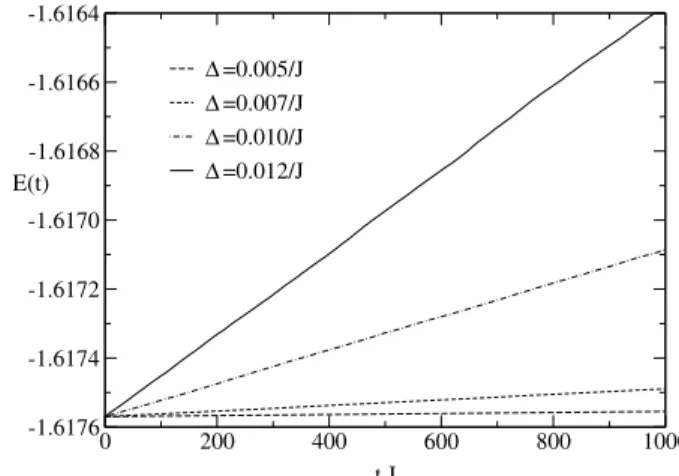
The performance of some of the algorithms discussed here will be illustrated with spin dynamics simulations of a Heisenberg ferromagnet on a 10x10x10 simple cubic lattice at temperatureT = 0.8Tc, whereTc is the critical temper-ature of the model. The equations of motion conserve both the total energy per siteE(t)and the uniform magnetization per site M(t) of the system. The fourth-order predictor-corrector method described above conserves the uniform magnetization exactly; however, the total energy drifts sys-tematically and considerably, even for relatively small time steps, as shown in Fig. 1.
0 200 400 600 800 1000
t J -1.6176
-1.6174 -1.6172 -1.6170 -1.6168 -1.6166 -1.6164
E(t)
∆ =0.005/J
∆ =0.007/J
∆ =0.010/J
∆ =0.012/J
Figure 1. Energy per site versus time obtained with the fourth-order predictor-corrector method for a single initial configuration using different time steps∆.
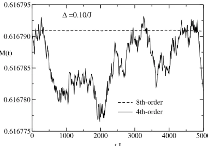
In contrast the decomposition algorithms conserve both energy and spin length exactly, because the scalar product of nearest-neighbor spins is preserved during the rotation of a spin around its effective field. The uniform magnetization is not exactly conserved by the decomposition algorithms; however, there is no long time drift in the magnetization, as illustrated in Fig. 2 for the fourth- and an eighth-order[6, 18] Suzuki-Trotter decomposition with∆ = 0.10/J. Note that the size of the integration step used here is almost an order of magnitude larger than the maximum∆in Fig. 1. More-over, the maximum integration time here istmax= 5000/J, which is a factor of 5 larger than in Fig. 1. Fig. 2 also shows that for the same time step, higher-order methods yield smaller magnetization fluctuations. The total fluctu-ation of the uniform magnetizfluctu-ation per site M(t) for the fourth- and the eighth-order method shown in Fig. 2 are ∼ 2×10⁻⁵ and∼ 2×10⁻⁷, respectively. Fig. 3 shows
0 1000 2000 3000 4000 5000 t J
0.616775 0.616780 0.616785 0.616790 0.616795
M(t)
8th-order 4th-order
∆ =0.10/J
Figure 2. Comparison of fluctuations in the uniform magnetiza-tion per site for the fourth- and an eighth-order Suzuki-Trotter decomposition with∆ = 0.10/J for a single initial configuration.
0 1000 2000 3000 4000 5000 t J
0.61674 0.61676 0.61678 0.61680 0.61682 0.61684
M(t)
∆ =0.10/J ∆ =0.20/J ∆ =0.25/J 8th-order
Figure 3. Comparison of fluctuations in the uniform magnetiza-tion per site for an eighth-order Suzuki-Trotter decomposimagnetiza-tion with different time steps∆for a single initial configuration.
0 1000 2000 3000 4000 5000 t J
0.61250 0.61300 0.61350 0.61400 0.61450
M(t)
FR
SZT
OFR
∆ =0.10/J
4th-order
Figure 4. Comparison of fluctuations in the uniform magnetization per site for three different 4th-order decomposition algorithms, namely Forest-Ruth (FR), Suzuki-Trotter (SZT) and an optimized Forest-Ruth (OFR) [see text], as a function of the integration time. A time step of∆ = 0.10/Jhave been used in all cases.
three cases the equations of motion were integrated out to
tmax = 5000/J, using a step of ∆ = 0.10/J. The FR method requires the fewer operations (rotations) per time
step; however, it also yields the largest magnetization fluc-tuation (∼ 2 ×10⁻³). In contrast, much smaller
fluctu-ations were observed with the SZT and the OFR methods (∼2×10⁻⁵in both cases).
Each integration step of the predictor-corrector method used here is approximately 2.5 times faster than each step using the fourth-order Suzuki-Trotter decomposition. How-ever, the latter generates results that are accurate for much larger time steps, and thus constitutes a much faster algo-rithm. Although the eighth-order method used here provides better magnetization conservation, it is not a very competi-tive algorithm because it requires a large number, namely 31, rotations per time step.
6.3
Further developments
Decompositions of exponential operators involving higher-order derivatives of the variables in the equations of motion, such as force gradients in the case of MD, have been im-plemented and shown to be more advantageous for some applications[19, 20, 21]. One such force-gradient decom-position is given by[21]
e(A+B)∆=
P
i=1
eaiA∆ebiB∆+ciC∆3+O(∆K+1) (41)
where
C≡[B,[A, B]] = N
i=1
gi
mi · ∂
∂vi
, (42)
gi= 2
k,k=i
jp,j=p
fjp
mj
∂fik
∂rjp
, (43)
andai,bi, andciare chosen to minimize the truncation er-rors.
For systems involving different time scales, decompo-sition methods can be used to integrate the slow varying components of the system with a larger time step than the rapidly varying components[22, 23]. As a simple example, let us consider an MD simulation where the Liouville op-erator can be separated into a slow and a rapidly varying part denoted asLsandLf, respectively. The second-order decomposition given by Eq.(35) can be further decomposed into
e(Lf+Ls)∆ = eLs∆2[eLfδ]neLs∆2 +O(∆3) (44)
whereδ= ∆/nis a smaller time step used to evolve the fast dynamics of the system.
Depending on the dynamics and types of interactions in the systems, it may be necessary to decompose the exponen-tial operator into more than two individual operators. For example, spin dynamics simulations of a spin system on a two-dimensional triangular lattice require a three-sublattice decomposition, and a second-order decomposition can be written as
e(A+B+C)∆= eA∆2eB ∆
2eC∆eB ∆ 2eA
∆
2 +O(∆3), (45)
where each of the three separate operatorseA∆,eB∆, and
on the other two sublattices fixed. Spin dynamics sim-ulations of an antiferromagnetic XY model on the tri-angular lattice have been done using a second-order de-composition algorithm[24]. The dynamic behavior of the model was studied for a range of temperatures, includ-ing around the Kosterlitz-Thouless transition and the Isinclud-ing transition, where long-range order appears in the staggered chirality[24]. There are several other applications studied in the literature that require decompositions involving multiple operators[25].
Finally, we remark that the sublattice decomposition re-quired for the implementation of decomposition algorithms allows a direct parallelization according to the shared mem-ory model (OpenMP) which results in essentially 100% par-allel code for, e.g., a spin dynamics integrator. This is partic-ularly interesting for many commercially available parallel clusters in which each node is often equipped with two pro-cessors on the main board sharing the installed main mem-ory. However, in practice one observes a severe reduction in parallel efficiency on many commercially available systems, e.g., the Intel Xeon, if the storage required to hold the lattice or the numerical grid of the problem exceeds the cache size of the processor. The reason for this is a lack of memory bandwidth in particular if CPU1 has to access the memory share of CPU2. In this case an additional chip set is invoked which performs a time consuming memory mapping opera-tion. We had the opportunity to make a few tests on an AMD Opteron node with two CPUs and the new Hypertransport architecture which makes one CPU essentially transparent for access to its memory share requested by the other CPU. It turns out that the parallel efficiency on this system remains on a high level independent of the lattice size which makes shared memory parallelism an efficient and easy-to-use tool to increase the turnaround also for simulations on memory consuming lattices in the future [26].
7
Spin dynamics results for RbMnF
3Spin dynamics of RbMnF3have been performed on simple
cubic lattices with linear sizes up to L = 72; this corre-sponds to solving a system of723= 373248equations[27].
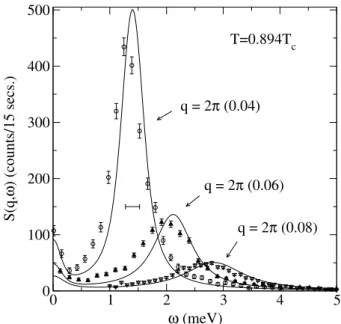
Direct comparisons of dynamic structure factorsS(q, ω)for momentumqand frequencyω obtained from spin dynam-ics simulations and neutron scattering data[28] yielded good quantitative agreement, with no adjustable parameters[11]. An illustration of this comparison atT = 0.894Tcfor mo-mentum transferqin the [111] direction is shown in Fig. 5. Integrations of the equations of motion were done up to tmax = 1000/J using the fourth-order Suzuki-Trotter decomposition given in Eq.(36) with a time step of∆ = 0.2/J. The experimental energy resolution width was0.25 meV, which is shown as a horizontal line segment in Fig. 5. For the direct comparison, dynamic structure factors from the simulations were convoluted with the experimental res-olution function and theT- andω-dependent population fac-tor was removed from the neutron scattering data. The nor-malization of the intensities ofS(q, ω)between simulation and experiment was done at oneT andq, the same factor was then used to normalize the curves for all values ofq.
0 1 2 3 4 5
ω (meV)
0 100 200 300 400 500
S(q,
ω
) (counts/15 secs.)
T=0.894Tc
q = 2π (0.04)
q = 2π (0.06)
q = 2π (0.08)
Figure 5. Comparison of dynamic structure factor as a function of frequency from simulation and experiment, for T = 0.894Tc
and q = (q, q, q). The symbols represent neutron scattering
data [the circles, triangles, and inverted triangles correspond to q = 2π(0.04), 2π(0.06), and2π(0.08), respectively] while the solid lines are simulation results forL= 60.
8
Summary
Molecular dynamics and spin dynamics simulations require good algorithms for the time integration of the equations of motion. Desirable properties of integration algorithms include accuracy for long time steps, time reversibility, good conservation of energy, and being symplectic (con-serve phase-space volume).
Standard integration algorithms in applied mathematics are, in general, neither time reversible nor symplectic, and they yield large long-term energy drift, unless very small time steps are used. In contrast, algorithms based on decom-position of exponential operators are time reversible, sym-plectic, and the energy fluctuations are bounded. In some cases the energy can be conserved exactly (within machine precision). In general, decomposition algorithms are also accurate for larger time steps and allow integration to much longer times thus allowing study of low frequency modes. These methods are broadly applicable and may be straight-forwardly applied to more complicated systems although more sublattices may be needed with a resultant increase in complexity.
Acknowledgments
References
[1] See e.g. M.P. Allen and D.J. Tildesley,Computer Simulation of Liquids, Oxford University Press 1987; D. Frenkel and B. Smit,Understanding Molecular Simulation, Academic Press 1996.
[2] D.P. Landau and M. Krech, J. Phys.: Condens. Matter 11, R179 (1999).
[3] H. Yoshida, Phys. Lett. A150, 262 (1990) [4] E. Forest and R.D. Ruth, Phys. D43, 105 (1990) [5] M. Suzuki, Phys. Lett. A165, 387 (1992).
[6] M. Suzuki and K. Umeno inComputer Simulation Studies in Condensed Matter Physics VI, edited by D.P. Landau, K.K. Mon, and H.-B. Sch¨uttler (Springer, Berlin, 1993).
[7] M.E. Tuckerman and G.J. Martyna, J. Phys. Chem. B104, 159 (2000).
[8] I.P. Omelyan, I.M. Mryglod, and R. Folk, Comput. Phys. Commun.151, 272 (2003).
[9] M. Krech, A. Bunker and D.P. Landau, Comput. Phys. Com-mun.111, 1 (1998).
[10] J. Frank, W. Huang, and B. Leimkuhler, J. Comput. Phys.
133, 160 (1997).
[11] S.-H. Tsai, A. Bunker, and D.P. Landau, Phys. Rev. B61, 333 (2000).
[12] See e.g., D.P. Landau and K. Binder, A Guide to Monte Carlo Simulations in Statistical Physics(Cambridge Univer-sity Press, 2000).
[13] See e.g. W.H. Press, S.A. Teukolsky, W.T. Vetterling, and B.P. Flannery,Numerical Recipes, the Art of Scientific Computing, second edition, Cambridge University Press, 1992.
[14] M. Suzuki, Prog. Theor. Phys.56, 1454 (1976).
[15] M. Suzuki, S. Miyashita, and A. Kuroda, Prog. Theor. Phys.
58, 1377 (1977).
[16] I.P. Omelyan, I.M. Mryglod, and R. Folk, Phys. Rev. E65, 056706 (2002).
[17] I.P. Omelyan, I.M. Mryglod, and R. Folk, Comput. Phys. Commun.146, 188 (2002).
[18] D.P. Landau, S.-H. Tsai, M. Krech, and A. Bunker, Int. J. Mod. Phys. C10, 1541 (1999).
[19] M. Suzuki, Phys. Lett. A201, 425 (1995).
[20] S.A. Chin, Phys. Lett. A226, 344 (1997).
[21] I.P. Omelyan, I.M. Mryglod, and R. Folk, Phys. Rev. E66, 026701 (2002).
[22] M. Tuckerman, B.J. Berne, and G.J. Martyna, J. Chem. Phys.
97, 1990 (1992).
[23] S.J. Stuart, R. Zhou, and B.J. Berne, J. Chem. Phys.105, 1426 (1996).
[24] K. Nho and D.P. Landau, Phys. Rev. B66, 174403 (2002).
[25] See e.g. I.P. Omelyan, I.M. Mryglod, and R. Folk, Phys. Rev. Lett.86, 898 (2001).
[26] M. Krech, unpublished.
[27] S.-H. Tsai and D.P. Landau, Phys. Rev. B67, 104411 (2003).