www.ocean-sci.net/11/779/2015/ doi:10.5194/os-11-779-2015
© Author(s) 2015. CC Attribution 3.0 License.
Estimation of upward radiances and reflectances at the surface
of the sea from above-surface measurements
Ø. Kleiv1, A. Folkestad1,a, J. Høkedal2, K. Sørensen1, and E. Aas3
1Norwegian Institute for Water Research, Gaustadalleen 21, 0349 Oslo, Norway 2Narvik University College, Lodve Langes gt. 2, 8505 Narvik, Norway
3Department of Geosciences, University of Oslo, Gaustadalleen 21, 0349 Oslo, Norway anow at: Rolls-Royce Marine Propulsion, Sjøgata 98, 6065 Ulsteinvik, Norway
Correspondence to:E. Aas ([email protected])
Received: 6 May 2015 – Published in Ocean Sci. Discuss.: 12 June 2015
Revised: 14 August 2015 – Accepted: 12 September 2015 – Published: 2 October 2015
Abstract. During 4 field days in the years 2009–2011, 22 data sets of measurements were collected in the inner Oslofjord, Norway. The data consist of recordings of spectral nadir radiances in air and water as well as spectral downward irradiance in air. The studied wavelengths are 351, 400, 413, 443, 490, 510, 560, 620, 665, 681, 709 and 754 nm.
The water-leaving radiance and the reflected radiance at the sea surface have been obtained from the measured nadir radiances in air and water, where the latter radiance has been extrapolated upwards to the surface. For comparison we present a simpler and much faster method that determines the water-leaving and reflected radiances solely from above-surface measurements of upward nadir radiance and down-ward irradiance. This new method is based on an assumption about similarity in spectral shape of the radiance reflected at the surface, and it makes use of the small ratio between water-leaving and reflected radiances at 351 and 754 nm in the Oslofjord.
A comparison between the quantities determined by the two mentioned methods shows that the average relative devi-ations between their results are less than or equal to 15 % for the reflected radiance, at the studied wavelengths. The aver-age relative deviation of the water-leaving radiance at 560 nm is 24 %. These results are obtained for a cloudiness range of 1–8 oktas (12.5–100 %) and solar zenith angles between 37 and 51◦. We consider these to be acceptable uncertainties for a first check of satellite products in the inner Oslofjord.
1 Introduction
The Norwegian Institute for Water Research (NIVA) has been monitoring the coastal waters of Norway by sensors in-stalled onboard ships on fixed and regular routes since 2001, in the FerryBox project and different ESA (European Space Agency) projects (Sørensen et al., 2007). The need for such monitoring rose during the period 1988–2001 when several toxic algal blooms occurred in the Skagerrak and resulted in severe losses for fish farms along the coast (see e.g. Kris-tiansen and Aas, 2015, and references therein). Monitoring is also an important part of obligations set out in the EU (Euro-pean Union) Water Framework Directive (2000/60/EC). The recordings of water quality can be coordinated with data from environmental satellites and used for validation pur-poses. The projects VAMP (Validation of MERIS (MEdium Resolution Imaging Spectrometer) Products), supported by the ESA (European Space Agency), and REVAMP (Regional Validation of MERIS Products), supported by the EU, are ex-amples of such satellite validation projects (Aas et al., 2005; Høkedal et al., 2005; Magnusson et al., 2003; Peters et al., 2005a, b; Sørensen et al., 2003, 2004, 2007). The MERIS L2 products to be validated in the mentioned projects were water-leaving reflectance, algae pigments index 2, total sus-pended matter, and the sum of yellow-substance absorption and bleached particle absorption.
at-mospheric contribution, but they have to be tilted in order to see a part of the sea surface that is not influenced by the ship. The recorded radiance will then be a function of the reflected sky radiance, the reflected direct radiance from the sun, the water-leaving radiance, the nadir angle of the field of view and the azimuth angle relative to the sun, as well as the wind speed. Doxaran et al. (2004) made above-surface recordings of the upward radiance from nadir,Lua(0◦), and at a nadir
angle of 40◦, Lua(40◦). The azimuth angle relative to the
solar plane was 135◦. During clear sky conditions the ratio
Lua(40◦) /Lua(0◦) varied in the ranges 0.9–2.2 and 0.6–2.6 at 450 and 850 nm, respectively. Under an overcast sky the ranges were 1.0–1.6 at both wavelengths. All of these factors constitute a challenge with regard to a quantitative analysis of the recordings (Bissett et al., 2004; Garaba and Zielinski, 2013; Hooker and Morel, 2003; Mueller et al., 2003; Simis and Olsson, 2013).
As a first step we have simplified the analysis and the prob-lem by reducing the number of nadir angles for the upward radiance to only one, 0◦, and we have investigated the pos-sibility of obtaining the spectral distribution of the water-leaving radiance solely from observations in air. The next step will then be to relate these results to recordings by sen-sors tilted at an angle from the nadir, so that recordings made by radiometric sensors mounted on ships of opportunity can be used directly for improved monitoring of water quality, estimation of water-leaving radiance and validation of satel-lite products. This step remains to be taken, and it is not de-scribed in this paper.
Descriptions of the applied instruments, the data sets of measurements and the environmental conditions are pre-sented in Sect. 2.1. A way of determining the water-leaving radiance as well as the radiance reflected upwards at the sur-face from recordings of the sub-sursur-face and above-sursur-face upward nadir radiances is outlined in Sect. 2.2, while a sim-pler method to estimate the reflected and water-leaving ra-diances from recordings in air is presented in Sect. 2.3. In Sect. 3.1 the constants necessary for the simple method are calculated, and finally the deviation between the two meth-ods is tested in Sect. 3.2.
2 Material and methods
2.1 Field measurements 2009–2011
The data discussed in this paper were collected during the years 2009–2011, as a part of the ESA supported VAMP II project. Data of the downward spectral irradiance in air,
Ed, the upward spectral radiance in air from nadir,Lua, and
the upward spectral radiance in water from nadir,Luw, will
be analysed. These radiometric quantities were recorded by sensors from the TriOS company: Ed by the sensor
Ram-ses AAC-VIS (diameter 4.83, length 26 cm), and Lua and Luwby Ramses ARC-VIS (diameter 4.83 cm, length 29.7 cm
plus spray protection cap 2.8 cm). Both sensors record by a silicon photodiode array consisting of 256 channels within the range 320–950 nm. The sensors were tested against the FieldCAL device from TriOS at the start of each field cruise. Data were recorded onboard the R/V Trygve Braarud and were stored in a laptop by the MSDA_XE software provided by TriOS. In the post-field processing of the data the wave-lengths were restricted to 351 nm and the OLCI (Ocean and Land Colour Instrument) channels planned for the Sentinel-3 satellite (ESA): 400, 41Sentinel-3, 44Sentinel-3, 490, 510, 560, 620, 665, 681, 709 and 754 nm. Except for 351 and 400 nm these cor-respond to the former MERIS wavebands. The Ramses chan-nels closest to the OLCI wavebands were chosen to represent the latter.
The irradiance sensor was mounted on a vertical pole above the roof of the ship bridge of the R/VTrygve Braarud, in order to avoid shading effects. The direction of the normal to the irradiance collector was assumed to be within 0–5◦ from the zenith. The radiance sensor was attached to a rig that measuredLuawhen the rig was suspended above the sea
surface andLuwwhen it was submerged in water. The
hori-zontal distance from the rig to the ship side was 3 m. Usually the recording depths in water were 0.5, 1, 1.5, 2, 2.5 and 3 m, corresponding to the well-mixed upper part of the water col-umn. The depths were determined by the length of a wire running over a meter wheel, and at each depth the recording periods (60 s) were chosen so as to average out the effects of waves. No ship roll was detected. The meter wheel was adjusted to zero when the radiance sensor passed the sea sur-face. The accuracy of the average depth was then probably better than 5 cm in most of our cases.
Altogether 22 data sets of Ed, Lua and Luw have been
analysed. The environmental conditions on the 4 field days are shown in Table 1, and the cloudiness shows that none of the days had a completely clear sky. Based on observations by the Norwegian Meteorological Institute from the last 10 years, the average cloudiness at 12:00 UTC in Oslo during May and June is 5.4 oktas. This means that on 3 of the 4 days in Table 1, the conditions were better than the average.
At each wavelength in each data set the median of the recorded data was applied in order to avoid the influence of spikes and other disturbances. The time series for a record-ing lasted for 60 s, and durrecord-ing that time around 14–38 tra could be recorded. In 2009 the average number of spec-tra was 22. Thus, we could say that the median is based on 26±12 values. However, usually the difference between mean and median values was not significant. In 2009 the vari-ation was greatest, as shown by Ed in Table 1. The
varia-tion ofLuais closely related toEd, and 40 % of theLuadata
had relative deviations between median and mean values less than 0.01, 37 % of the data had deviation in the range 0.01– 0.05, 16 % had deviations in the range 0.05–0.10, while only 7 % had deviations above 0.10.
For each data set the ratio (Ed(max)–Ed(min)) /Ed(mean)
Table 1.Environmental conditions during field work at 59◦49′N, 10◦34′E.
Date Wind Cloudiness Mean Solar Number Range/mean speed cloudiness zenith of series ofEd
(m s−1) (oktas) (oktas) angle (◦) at 560 nm 25 June 2009 2.8 1–3 1.7 37–50 9 0.01–1.17 6 May 2010 2.5 4–8 6.3 43–44 3 0.09–0.43 7 May 2010 4.9 2–3 2.3 43–51 7 0.01–0.36 10 May 2011 2.3 4–6 5.3 45–50 3 0.02–0.33
lower and upper value, as displayed by Table 1. We see that the ratio could vary between 0.01 and 1.17, meaning a highly variable downward irradiance. Because a median filter had already been used on the recordings, the variation is not a result of sudden shifts but a result of major changes in the irradiance conditions.
The wind speeds, however, were favourable during the 4 field days, being<5 m s−1. In 2011 the sea showed signifi-cant patches of pollen, which do not seem to have influenced the recordings.
The recordings were made in yellow-substance-rich coastal waters near the islands of Steilene in the inner Oslofjord. The bio-optical properties of this area have been presented by Aas et al. (2005), Høkedal et al. (2005) and Sørensen et al. (2003, 2004, 2007). While the annual range of the Secchi disk depth at this location stretches from 2 m during vernal algal bloom to 12 m under winter conditions (Aas et al., 2014), the Secchi disk depths on the 4 days in Ta-ble 1 were in the range of 5.0–6.5 m. The content of yellow substance or CDOM (Coloured Dissolved Organic Material) can be quantified by its absorption coefficient at 442 nm. The mean value±the standard deviation of the coefficient at this wavelength, based on data mainly from the Skagerrak and the Oslofjord is 0.62±0.60 m−1, according to Sørensen et
al. (2007).
2.2 Processing ofLuwmeasurements
The radiance from the nadir in water,Luw(z), is a function of
the vertical coordinate z, defined positive downwards from the surface. We assume that this function can be approxi-mated by a relationship on the form
Luw(z)=Luw(0) e−Kz (1)
for monochromatic radiance.Kis the vertical attenuation co-efficient of the radiance (Jerlov, 1976), and it is assumed to be practically constant. Usually the upper 3 m were well mixed. Due to surface waves it is not possible to measure the ra-diance valueLuw(0) just beneath the surface with sufficient
accuracy, but it can be estimated by linear regression analysis of the expression
ln(Luw(z))=ln(Luw(0))−Kz, (2)
where ln(Luw(z))andz are the variables. Experience
con-firms that Eq. (2) describes the vertical attenuation of the radiance Luw(z) fairly well, provided the light conditions
in the atmosphere remain constant during the recording. If, on the other hand, the downward irradianceEdin air varies significantly, we have no perfect method to compensate for this. The best way may be to choose a reference valueEd, ref
for the irradiance among those values observed during the recording ofLuw(z), and then estimate corrected values of
Luw(z)at the different depths by assuming
Luw,corr
Ed,ref
≈Luw(z)
Ed , (3)
whereEdis the observed irradiance at the time whenLuw(z)
was recorded.
The recordings ofLuwshould not be made too close to the
ship’s side. Korsbø and Aas (1997) investigated the influence of ship-shading on upward radiance onboard the R/VTrygve Braarudin the Oslofjord. The size of the ship is length 22 m, width 7 m, keel depth 3 m and bridge 6 m above sea surface. Recordings just behind the stern of the ship, with the sun on the same side, could typically be reduced by up to 20 %, while recordings at a distance of 5 m did not seem to be in-fluenced by the ship. In the present case the distances have been 3 m, on the sunlit side of the ship, and the influence of the ship has been assumed negligible.
While the superstructure of the ship will prevent some of the sky radiance to reach the part of the surface that the radi-ance sensor is observing, it may also reflect direct solar and diffuse sky radiation towards the same area. This will influ-ence the value ofLw. The problem has been discussed by
Hooker and Morel (2003) and Hooker and Zibordi (2005). In our case we find that this reflectance was included in the ship-shading effect determined by Korsbø and Aas (1997).
Another possible source of error is the self-shading effect of downward-looking instruments in the sea. Gordon and Ding (1992) used Monte Carlo simulations to describe this effect, and Zibordi and Ferrari (1995) tested their results by field measurements. Korsbø quantified the self-shading effect in the Oslofjord by in situ measurements (Aas and Korsbø, 1997). The effect was described by
ln(1−ε)=ln
L
uw, meas Luw, true
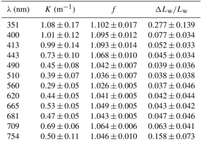
Table 2.Mean value±standard deviation of the vertical attenuation coefficientKof sub-surface radiance from nadir, of the correction factor f for self-shading by the radiance sensor, and of the rela-tive uncertainty1Lw/Lwof the water-leaving radiance at different
wavelengthsλ. The number of analysed data sets is 22.
λ(nm) K(m−1) f 1Lw/Lw
351 1.08±0.17 1.102±0.017 0.277±0.139 400 1.01±0.12 1.095±0.012 0.077±0.034 413 0.99±0.14 1.093±0.014 0.052±0.033 443 0.73±0.10 1.068±0.010 0.045±0.034 490 0.45±0.08 1.042±0.007 0.039±0.036 510 0.39±0.07 1.036±0.007 0.038±0.038 560 0.29±0.05 1.026±0.005 0.037±0.046 620 0.44±0.05 1.041±0.005 0.042±0.044 665 0.53±0.05 1.049±0.005 0.043±0.042 681 0.47±0.05 1.043±0.005 0.047±0.046 709 0.69±0.06 1.064±0.006 0.063±0.041 754 0.50±0.11 1.046±0.010 0.158±0.073
where ε is the relative error of the measured radiance
Luw, meas, andLuw, trueis the true radiance.Bis a function of wavelength and solar zenith angle, and Korsbø determined its value by correlation analysis between the variablesrand
Luw,meas. The radiance sensor has the shape of a cylinder, andris its radius.Kis the vertical attenuation coefficient of the nadir radiance (Jerlov, 1976). From Eq. (4) the correction factorf (λ)=Luw, true/Luw, measmay be written
f (λ)= Luw, true Luw, meas =e
BKr. (5)
Based on the solar angles in Table 1 and the results of Aas and Korsbø (1997), we have estimated a mean value of the dimensionlessB in Eq. (5) equal toB=(2.5±0.6) for all wavelengths. Combined with the dimensions of the TriOS ra-diance sensor described in Sect. 2.1, the corresponding value of the productBrbecomesBr=(0.09±0.01) m. The mean values and standard deviations ofKandf (λ), based on all 22 data sets of observation forzin the depth range 0.5–3.0 m, are presented in Table 2 at 351 and 400 nm and the MERIS spectral channels in the range 413–754 nm. It illustrates that if the self-shading effect is not taken into account, the ex-trapolated value ofLuw(0) found by Eq. (4) will on average be underestimated by 3–9 % in the Oslofjord by the Ramses-ARC sensor. It should be noted that the small signals pro-duced by the radiance Luw(z) at the smallest and greatest
wavelengths increase the uncertainty of the estimatedKand
f (λ)at these wavelengths.
When Luw, meas(0) has been multiplied by the correction
factor f, resulting inLuw, true(0) according to Eq. (5), the
transmittance process through the surface has to be consid-ered. This transmittance is first influenced by Fresnel reflec-tion at the surface and then by Snell refracreflec-tion when the ra-diance enters the air. The first process reduces the rara-diance
by loss of energy flux, and the second process reduces the radiance by spreading the flux into a greater solid angle. The water-leaving radianceLw is obtained by multiplying Luw, true(0) by the transmittance of nadir radiance through the
surface from water to air,CL:
Lw=CLLuw, true(0). (6)
Because this value for the water-leaving radiance is based on in-water measurements, we will denote it asLw, meas. By
inserting forLuw, true(0) from Eq. (5), Eq. (6) may then be
written
Lw, meas=CLf (λ)Luw, meas(0). (7)
Austin (1974) assumed a constant refractive index of sea-water and obtained the value 0.543 for CL, while Aas et
al. (2009) suggested the approximated value 0.546 for the Oslofjord. The factor can also be determined more precisely by a formula taking into account the wavelength λ, the sea temperatureT and the salinityS(Aas et al., 2009). For
T ≈10◦C andS≈20, the formula becomes
CL≈0.5458+0.00003855(λ−550), (8) whereλis in nanometres. Our values ofCLwere calculated
by this formula.
The radiance sensor was also used in air at a height of 1– 2 m above the surface to record the total upward radianceLua
above the same water mass that producedLw. The radiance
meter in air receives light from a greater solid angle than in water and consequently a different calibration, provided by the TriOS company, has to be applied. The calibration fac-torFwfor the instrument in water, relative to the calibration factorFain air, is (e.g. Aas, 1994)
Fw Fa =
n
g+nw ng+1
2
nw. (9)
Hereng andnw are refractive indices of the glass window of the radiance meter and the seawater, respectively. They are functions of wavelength, and between 351 and 900 nm the ratioFw/ Fa will vary from 1.774 to 1.722 (Ohde and
Siegel, 2003; see also Zibordi and Darecki, 2006). 2.3 Estimation of reflectance at the surface fromLua
andEd
The total upward nadir radianceLua in air consists of two
terms; the Fresnel-reflected upward radiance at the surface
Lrand the water-leaving radianceLw:
Lua=Lr+Lw. (10)
When the water-leaving radiance Lw has been determined
from Eq. (7), the upward reflected radianceLrat the surface
0 0.002 0.004 0.006 0.008 0.01 0.012 0.014
350 450 550 650 750 850
Wavelength (nm) Rr,m
eas
(sr
-1)
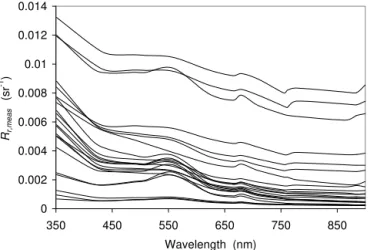
Figure 1.Spectral distribution of the measured radiance reflectance
Rr, meas.
section that the superstructure of the ship in general may re-flect direct solar and diffuse sky radiation towards the field of view of the radiance sensor and thus influence the values of
LrandLw, but it was also concluded that we think that this
effect is negligible in our case.
If there is no wind and the surface is flat, the value ofLr
can be estimated from Lr≈0.021Ld, whereLd is the sky radiance from zenith and 0.021 is the value of the Fresnel reflectance for normal incidence at the air–water interface. However, if some wind is present, the estimate of Lr from
the zenith radiance can lead to significant errors. Aas (2010) found that the contributions from the sun and the diffuse sky to Lr had to be calculated separately, and polynomials for
these calculations were presented. Unfortunately, the poly-nomials require a clear sky, which is not the condition on our field days, as seen by Table 1. Accordingly, we need a differ-ent method to estimateLr.
By dividing Eq. (10) byEd, it can be rewritten as
Rua=Rr+Rw, (11)
whereRua(λ),Rr(λ)andRw(λ)represent the spectral
radi-ance reflectradi-ances
Rua(λ)= Lua(λ)
Eda(λ), (12)
Rr(λ)= Lr(λ) Eda(λ)
, (13)
Rw(λ)=Lw(λ) Eda)
. (14)
Rwis often termed the remote sensing reflectance, as well as
the water-leaving reflectance.
By comparing the spectral distributions ofLr(λ)andRr(λ)
we have noticed that the spectral shape ofRr(λ)is more
con-stant than the shape ofLr(λ). Consequently we will base our
estimation method on an analysis ofRr(λ). Figure 1 presents
0.4 0.5 0.6 0.7 0.8 0.9 1
350 450 550 650 750 850
Wavelength (nm) Lr,
m
ea
s
/Lua
Figure 2.Spectral distribution of the ratioLr, meas/ Lua.
Rr(λ)for our data. If we regardRr(754) as a baseline, and the
differenceRr(351)−Rr(754) as a scaling factor, we may be
able to describe the spectral shape ofRr(λ)–Rr(754) within the interval 351–754 nm by
Rr(λ)−Rr(754)=A(λ)[Rr(351)−Rr(754)], (15)
whereA(λ) is a constant of proportionality. The value of
A(λ) can be calculated by determining the best-fit line through the origin for Rr(λ)−Rr(754) as a function of Rr(351)−Rr(754), with the spectral curves of Fig. 1 as input.
The results will be presented for the MERIS/OLCI wave-lengths in Sect. 3.1.
Equation (15) definesRr(λ)as a function of the two vari-able spectral endpointsRr(351) andRr(754) and the shape factorA(λ). The reflectancesRr(351) andRr(754) have been obtained from in-water recordings of Luw combined with recordings in air ofEd, and accordingly we should search for a method to estimate these reflectances solely from our above-surface recordings. If we transform Eq. (10) to
Lr Lua
=1−Lw Lua
, (16)
this form of the equation gives the useful information that
Lr/Lua, ≈1 at wavelengths whereLw/Lua≪1, and we would expect that this was true in the UV and red parts of the spectrum. Ruddick et al. (2006) have pointed out that the spectral shape ofRw=Lw/Edin the near-infrared part of
the spectrum tends to be invariant, because it is dominated by the strong absorption by pure water. This will also influence the spectral shape ofRua. Yellow substance will reduceRwin
the UV. The measured spectral distribution ofLr(λ)/Lua(λ)
is presented in Fig. 2.
We see that at 351 and 754 nm the ratio Lr/Lua= Rr/Ruacomes much closer to 1 than in the central part of
0 0.002 0.004 0.006 0.008 0.01 0.012 0.014
0 0.002 0.004 0.006 0.008 0.01 0.012 0.014
Rua
Rr 351
754
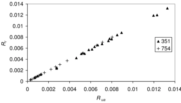
Figure 3.The upward radiance reflectance in air,Rr, as a function
of the total upward reflectance in air,Rua, at 351 and 754 nm.
recordings, the result may be written
Rr(351)≈C(351)Rua(351), (17)
whereC(351) is the slope of the line. A similar procedure at 754 nm gives
Rr(754)≈C(754)Rua(754). (18)
Figure 3 presentsRras a function ofRuaat 351 and 754 nm.
Clearly, the deviations from a line through the origin with a slope of 1 are small. By inserting from Eqs. (17) and (18) in Eq. (15), we obtain a relationship forRr(λ)where the only variable input is the value ofRuaat 351 and 754 nm:
Rr(λ)=A(λ)C(351)Rua(351)+[1−A(λ)]C(754)Rua(754).
(19)
2.4 Uncertainties ofLua,LwandLr
In Sect. 2.1 it was pointed out that the relative differences between our applied median and mean values ofLuain 2009
were less than 5 % for 77 % of the data. In the other years with more stable irradiance conditions the deviations are as-sumed to have been even less. The calibration of the sen-sors introduces uncertainties of a similar magnitude. It was mentioned in Sect. 2.1 that the radiance and irradiance sen-sors were calibrated against the FieldCAL device before each field cruise. According to the TriOS company the applied sensors have an “accuracy better than 6 %, depending on spectral range”. Based on the magnitude ofLuain the
differ-ent parts of the spectrum, and the quality of the field record-ings, expressed by the difference between mean and median values, we have estimated that the relative uncertainty ofLua
may be around 3 % in the central parts of the studied spec-trum,
Because the water-leaving radianceLw is obtained from
the extrapolated nadir radianceLuw(0) just beneath the
sur-Table 3.Best-fit values ofAin the range 400–709 nm, ofCat 351 and 754 nm, and the rms deviations between these values and indi-vidual calculations ofAandCat the wavelengthsλ.
λ(nm) AorC rms
351 0.977 0.039 400 0.661 0.047 413 0.567 0.060 443 0.470 0.078 490 0.444 0.139 510 0.433 0.156 560 0.429 0.248 620 0.198 0.095 665 0.129 0.061 681 0.147 0.079 709 0.078 0.039 754 0.993 0.031
face by Eq. (7), the relative uncertainty1Lw/ Lwcan be ap-proximated by the similar uncertainty1Luw(0)of the
radi-ance extrapolated to the surface by Eq. (2). If we write Eq. (2) as y=y0+Kz, where y=ln(Luw(z) and y0=ln(Luw(0)),
then the statistical expression for the standard deviationsy0
ofy0is
sy0= KL
r
1−r2 N−2z
2
0.5
, r=KL sz
sy
, (20)
whereris the correlation coefficient,Nis the number of ap-plied depths, usually 6, andsyis the standard deviation ofy. The average values ofsy0/ y0=1Lw/ Lw are presented in
Table 2, and at most of the wavelengths the relative uncer-tainty is less than 5 %. Based on these estimates, we have assumed that the relative uncertainty of the measured Lw
may be around 4 % in the central parts of the studied spec-trum, and that the uncertainty of the measuredLr, depending
on Lua as well as Lw, may be around 5 %. At the border
wavelengths, 351 and 754 nm, the uncertainty ofLwmay be
greater by a factor of 4–8, as indicated in Table 2.
3 Results
3.1 Values ofAandC
The spectral values ofA(λ)in Eq. (15) have been calculated as described in Sect. 2.3, with the spectral curves of Fig. 1 as input. The results are presented for the OLCI wavelengths between 400 and 709 nm in Table 3. Similarly, the values ofC(351) andC(754) were found by determinations of the best-fit lines for Eqs. (17) and (18), and the results are shown in Table 3.
y = 0.984x
0 0.002 0.004 0.006 0.008 0.01 0.012
0 0.002 0.004 0.006 0.008 0.01 0.012
Rr,meas (sr -1
) Rr,e
s
t
(sr
-1)
Figure 4.Estimated vs. measured values of the radiance reflectance
Rrfor all data sets and wavelengths.
of AandC in Table 3 are presented in the last row of Ta-ble 3. At 560 nm the deviations constitute more than 50 % of the calculated value ofA. Fortunately, the accuracy of the es-timated radiances is far better than the rms values in Table 3 might suggest. This will be demonstrated in the next section. 3.2 Estimates ofRr,Lr,RwandLw
We will denote the estimates ofRrprovided by Eqs. (17)– (19) as Rr, est. These may then be compared to the values
Rr, meas obtained from the field measurements of Luw,Lua
andEd. The result is shown in Fig. 4 for the OLCI channels in the range 400–754 nm with the addition of 351 nm. The best-fit line trough the origin obtains the slope 0.984, which is close to 1.
The root-mean-square deviations between Rr, est and Rr, measare presented for the different wavelengths in Table 4.
The rms deviations relative to the mean values are ≤13 %. We think this is a satisfactory result when the intention is to use the estimates as a first check of satellite products.
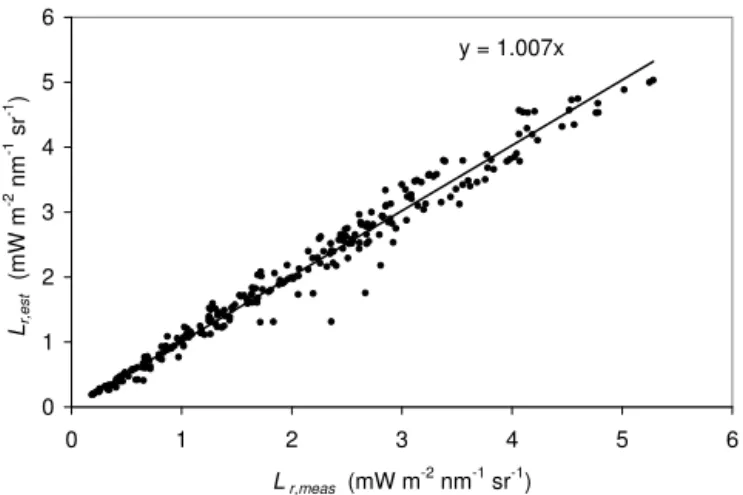
If we multiply Eqs. (17)–(19) by Ed(λ), we obtain the
estimates Lr, est(λ) at the different wavelengths. These re-sults can be compared to the corresponding measured val-uesLr, meas(λ). Figure 5 presents the estimated vs. the mea-sured reflected radiances. Again, the best-fit line obtains a slope close to 1.007. The relative rms deviations forLr are only slightly greater than the corresponding deviations for
Rr, namely≤15 %, as demonstrated by Table 4. At 351 and
754 nm the deviations between estimated and measured val-ues ofLr are only 3 and 1 %, respectively, because at these
wavelengths the water-leaving radiance in the Oslofjord be-comes so small that the recorded value ofLuacomes close
toLr, orRuaclose toRr. An important point here is that the
estimate ofLris not obtained from a measured sky radiance
multiplied by a Fresnel type of reflection coefficient, depend-ing on the sea roughness, but from the constants A andC
and the measuredLuaandEd. We assume that this method is
y = 1.007x
0 1 2 3 4 5 6
0 1 2 3 4 5 6
Lr,meas (mW m -2
nm-1 sr-1) Lr,e
s
t
(mW m
-2 nm -1 sr -1 )
Figure 5.Estimated vs. measured values of the reflected radiance
Lrfor all data sets and wavelengths.
Table 4.Mean values of measured radiance reflectanceRr, measand
reflected radianceLr, meas, and the rms deviations between these
quantities and the corresponding estimated values.
λ Rr, meas Lr, meas
mean rms meanrms mean rms meanrms
(nm) (10−5sr−1) (%) (10−2mW m−2nm−1sr−1) (%)
351 615 17 2 157 4.5 3
400 477 21 4 229 10 4
413 438 25 6 249 13 5
443 400 23 6 264 16 6
490 393 29 7 276 24 9
510 389 32 8 277 27 10
560 391 50 13 274 42 15
620 289 27 9 172 18 10
665 260 22 9 144 14 9
681 268 27 10 144 16 11
709 237 20 8 117 11 9
754 205 2.1 1 88 1.3 1
valid for solar zenith angles in the range 37—50◦and wind speeds up to 5 m s−1in the Oslofjord.
According to Eq. (11) we will obtain the estimate
Rw, est(λ)by subtractingRr, est(λ)fromRua(λ). The estimates
of this quantity at 351 and 754 nm can be obtained by com-bining Eqs. (11) and (17)–(18) with the results of Table 3. The results are
Rw, est(351)=(1−0.977)Rua(351)=0.023Rua(351), (21) and
Rw, est(754)=(1−0.993)Rua(754)=0.007Rua(754). (22) The estimated vs. the measured values ofRwat 351 nm and
y = 1.028x
0 0.001 0.002 0.003 0.004 0.005
0 0.001 0.002 0.003 0.004 0.005
Rw,meas (sr-1)
Rw,es
t
(sr
-1 )
Figure 6.Estimated vs. measured values of the remote sensing re-flectanceRwfor all data sets and wavelengths.
Table 5. Mean values of measured remote sensing reflectance
Rw, meas and water-leaving radianceLw, meas, and the rms
devia-tions between these quantities and the corresponding estimated val-ues.
λ Rw, meas Lw, meas
mean rms meanrms mean rms meanrms
(nm) (10−5sr−1) (%) (10−2mW m−2nm−1sr−1) (%)
351 19 17 89 5.2 4.5 87
400 71 21 29 39 10 25
413 74 25 33 48 13 28
443 97 23 24 74 16 21
490 146 29 20 120 24 20
510 164 32 19 137 27 20
560 213 50 24 173 42 24
620 95 27 28 71 18 25
665 62 22 36 45 14 30
681 67 27 40 46 16 35
709 32 20 63 21 11 52
754 2.9 2.1 72 1.6 1.3 80
Rr, est(λ), because Eq. (11) links the two quantities together,
andRuais the same for both the estimated quantities. In Ta-bles 4 and 5 the rms values are equal forRrandRw, but the ratio between the rms and the mean value becomes greater forRwthan forRr, because the mean values ofRware much smaller than the corresponding values ofRr.
If we multiply the estimatesRw, est(λ) byEd(λ), we ob-tain the estimatesLw, est(λ), which again can be compared to
the measuredLw, meas(λ). Figure 7 presents the estimated vs.
the measured water-leaving radiances, and the best-fit line has the slope 0.995. At 560 nm, where the water-leaving ra-diance has its peak value, the relative rms deviation is 24 % (Table 5), which we think is a surprisingly low value, consid-ering the uncertainties involved. We also consider this rms deviation to be a realistic example of what can be achieved in our waters. Hooker and Zibordi (2005) refer to an accuracy of 5 % required by NASA (National Aeronautics and Space
y = 0.995x
0 1 2 3 4 5
0 1 2 3 4
Lw,meas (mW m -2
nm-1 sr-1) Lw,est
(m
W m
-2 nm -1 sr -1)
Figure 7.Estimated vs. measured values of the water-leaving radi-anceLwfor all data sets and wavelengths.
Table 6.Values ofAandCand the measured radiance reflectance
Rr, meas at 560 nm for all data sets taken together and for the test
case withAandCdetermined from 9 data sets and applied on the remaining 13 data sets. The rms represents the deviations between
Rr, measand the corresponding estimated values ofRr, est.
Number C(351) A(560) C(754) Rr, meas(560)
of data sets mean rms meanrms
(10−5sr−1) (%)
22 0.977 0.429 0.993 391 50 13
9 selected 0.955 0.488 0.990 390 63 16
13 extra 392 48 12
Administration) for ground truth measurements, but this we think can only be achieved under very favourable conditions. It could be argued that because we have calculated the de-viations by the same data set that was applied for the best-fit constants, the test on an independent data set might produce greater deviations. Accordingly, we have tried to make such tests by dividing our data sets into two parts: one for the de-termination of the constantsAandC, and one for the cal-culation of deviations between measured and estimated re-flectances. As an example, the 9 sets from 2009 have been selected for the determination ofA andC, and then these values have been applied to the remaining 13 sets from 2010 to 2011. The results for the radiance reflectanceRrat 560 nm
are presented in Table 6. We find that the results for all sets together or for the sets divided into two parts are not signifi-cantly different.
4 Summary and conclusions
cor-responding upward radiance Lua in air, and the downward
irradianceEdin air. Comments on the data, the applied
sen-sors and the environmental conditions have been presented in Sect. 2.1.
Section 2.2 describes how the water-leaving radianceLw
and the reflected radiance Lr at the sea surface are
deter-mined fromLuaandLuw. A simpler and much faster method,
which determines the reflectanceRr=Lr/ Edas well asLr
andLwsolely from the measurements in air ofLuaandEd,
is presented in Sect. 2.3. The coefficientsAandC, defined by Eqs. (15) and (17)–(18), are key parts of this method, and they are quantified in Sect. 3.1. The applied wavelengths are 351 nm in addition to the 11 OLCI channels in the range 400– 754 nm.
A comparison between the quantities determined by the two methods shows that the average relative deviations be-tween their results are less than or equal to 13 and 15 % forRrandLr, respectively (Sect. 3.2). The deviations of the
water-leaving radianceLwand the corresponding reflectance Rw=Lw/ Edare identical to those ofRrandLrwhen
mea-sured in absolute units, but in relative units they become greater because Rw andLw are smaller thanRrandLr. On
the other hand, at 560 nm where Lw obtains its maximum
values, the average relative deviation between the two meth-ods is still only 24 % for bothRw andLw, and we consider
this to be an acceptable uncertainty of the estimates. These results have been obtained for a cloudiness range of 1–8 oktas and solar zenith angles between 37 and 51◦.
Our overall conclusion is that the suggested method to es-timate reflected and water-leaving radiances, based on mea-surements in air of upward nadir spectral radiance and down-ward spectral irradiance, provides results with a satisfactory accuracy. The remaining task is to determine the relation-ships between radiance from nadir and radiance recorded by tilted sensors. The recordings made by radiometric sensors mounted on ships of opportunity can then be used for a first check of the remote sensing reflectance estimated by satel-lites, at significantly lower costs than those required by the use of research vessels.
Author contributions. All authors participated in parts of the field work. Post-field processing of the data was made by Folkestad and Kleiv. Sørensen directed the project. Aas prepared the manuscript with comments and data from the co-authors.
Acknowledgements. The field work and the first processing of the data was part of the PRODEX project C90383 Validation of MERIS products – VAMP II, supported by ESA. A minor part of the data processing was supported by the Department of Geosciences at the University of Oslo.
Edited by: O. Zielinski
References
Aas, E.: A simple method for radiance calibration, in: European workshop on optical ground truth instrumentation for the valida-tion of space-borne optical remote sensing data of the marine en-vironment 23–25 November 1993, Netherlands Institute for Sea Research, Rep. 1994-3, 39–44, 1994.
Aas, E.: Estimates of radiance reflected towards the zenith at the surface of the sea, Ocean Sci., 6, 861–876, doi:10.5194/os-6-861-2010, 2010.
Aas, E. and Korsbø, B.: Self-shading effect by radiance meters on upward radiance observed in coastal waters, Limnol. Oceanogr., 42, 968–974, 1997.
Aas, E., Høkedal, J., and Sørensen, K.: Spectral backscattering coef-ficient in coastal waters, Int. J. Remote Sens., 26, 331–343, 2005. Aas, E., Høkedal, J., and Højerslev, N. K.: Conversion of sub-surface reflectances to above-sub-surface MERIS reflectance, Int. J. Remote Sens., 30, 5767–5791, 2009.
Aas, E., Høkedal, J., and Sørensen, K.: Secchi depth in the Oslofjord-Skagerrak area: theory, experiments and relationships to other quantities, Ocean Sci., 10, 177–199, doi:10.5194/os-10-177-2014, 2014.
Austin, R. W.: The remote sensing of spectral radiance from below the ocean surface, edited by: Jerlov,N. G. and Steeman Nielsen, E., Optical Aspects of Oceanography, Academic Press, London, 317–344, 1974.
Bissett, W. P., Arnone, R. A., Davis, C. O., Dickey, T. D., Dye, D., Kohler, D. D. R., and Gould, J., R. W.: From meters to kilome-ters: A look at ocean-color scales of variability, spatial coher-ence, and the need for fine-scale remote sensing in coastal ocean optics, Oceanography, 17, 32–43, 2004.
Doxaran, D., Nagur Cherukuru, R. C., and Lavender, S. J.: Esti-mation of surface reflection effects on upwelling radiance field measurements in turbid waters, J. Opt. A, 6, 690–697, 2004. Garaba, S. P. and Zielinski, O.: Methods in reducing
sur-face reflected glint for shipborne above-water remote sens-ing, J. Europ. Opt. Soc.-Rap. Publ., 8, 13058, 8 pp., doi:10.2971/jeos.2013.13058, 2013.
Gordon, H. R. and Ding, K.: Self-shading of in-water optical instru-ments, Limnol. Oceanogr., 37, 491–500, 1992.
Hooker, S. B. and Morel, A.: Platform and environmental effects on above-water determinations of water-leaving radiances, J. At-mos. Oceanic Techn., 20, 187–205, 2003.
Hooker, S. B. and Zibordi, G.: Platform perturbations in above-water radiometry, Appl. Opt., 44, 553–567, 2005.
Høkedal, J., Aas, E., and Sørensen, K.: Spectral optical and bio-optical relationships in the Oslo Fjord compared with similar results from the Baltic Sea, Int. J. Remote Sens., 26, 371–386, 2005.
Jerlov, N. G.: Marine Optics, Elsevier, Amsterdam, 1976.
Korsbø, B. and Aas, E.: Ship-shading effects on upward radiance and irradiance in coastal waters, Rep. Dept. Geophys., Univ. Oslo, 101, 13 pp., 1997.
Kristiansen, T. and Aas, E.: Water type quantification in the Skager-rak, the Kattegat and off the Jutland west coast, Oceanologia, 57, 177–195, 2015.
Mueller, J. L., Davis, C., Arnone, R., Frouin, R., Carder, K., Lee, Z. P., Steward, R. G., Hooker, S., Mobley, C. D., and McLean, S.: Above-water radiance and remote sensing reflectance mea-surement and analysis protocols, in: Ocean Optics Protocols For Satellite Ocean Color Sensor Validation, Revision 4, Volume III: Radiometric Measurements and Data Analysis Protocols, NASA/TM-2003-21621/Rev-Vol. III, 21–31, 2003.
Ohde, T. and Siegel, H.: Derivation of immersion factors for the hy-perspectral TriOS radiance sensor, J. Opt. A, 5, L12–L14, 2003. Peters, S. W. M., Eleveld, M., Pasterkamp, R., van der Woerd, H., Devolder, M., Jans, S., Park, Y., Ruddick, K., Block, T., Brock-mann, C., Doerffer, R., Kraseman, H., Röttgers, R., Schönfeld, W., Jørgensen, P. V., Tilstone, G., Martinez-Vincente, V., Moore, G., Sørensen, K., Høkedal, J., Johnsen, T. M., Lømsland, E. R., and Aas, E.: Atlas of Chlorophyll-a concentration for the North Sea based on MERIS imagery of 2003, Vrije Universiteit, Ams-terdam, 121 pp., 2005a.
Peters, S., Brockmann, C., Eleveld, M. , Pasterkamp, R., van der Woerd, H., Ruddick, K., Park, Y., Block, T., Doerffer, R., Krase-mann, H., Roettgers, R., Schoenfeld, W., Joergensen, P., Tilstone, G., Martinez-Vicente, V., Moore, G., Soerensen, K., Hokedal, J., and Aas, E.: Regional chlorophyll retrieval algorithms for North Sea waters: intercomparison and validation. Proceedings of the MERIS (A)ATSR Workshop 2005 (ESA SP-597), 26– 30 September 2005 ESRIN, Frascati, Italy, edited by: Lacoste, H.. Published on CDROM, p. 19.1 Publication Date: 12/2005, 2005b.
Ruddick, K. G., De Cauwer, V., Park, Y., and Moore, G.: Seaborne measurements of near infrared water-leaving reflectance: The similarity spectrum for turbid waters, Limnol. Oceanogr., 51, 1167–1179, 2006.
Simis, S. G. H. and Olsson, J.: Unattended processing of shipborne hyperspectral reflectance measurements, Rem. Sens. Environ., 135, 202–212, 2013.
Sørensen, K., Høkedal, J., Aas, E., Doerffer, R., and Dahl, E.: Early results for validation of MERIS water products in the Skagerrak. Proceedings of “Envisat Validation Workshop”, 9–13 December 2002, Frascati, Italy (ESA SP-531, March 2003), 2003. Sørensen, K., Aas, E., Høkedal, J., Severinsen, G., Doerffer, R., and
Dahl, E.: Validation of MERIS water products in the Skagerrak. MAVT Workshop. Proceedings of Envisat Validation Workshop, 20–24 October 2003, Frascati, Italy (ESA CD-ROM), 2004. Sørensen, K., Aas, E., and Høkedal, J.: Validation of MERIS water
products and bio-optical relationships in the Skagerrak, Int. J. Remote Sens., 28, 555–568, 2007.
Zibordi, G. and Darecki, M.: Immersion factors for the RAMSES series of hyper-spectral underwater radiometers, J. Opt. A, 8, 252, doi:10.1088/1464-4258/8/3/005, 2006.